River Buffer and HAND Exposure Analysis for the Maldevta Song Watershed
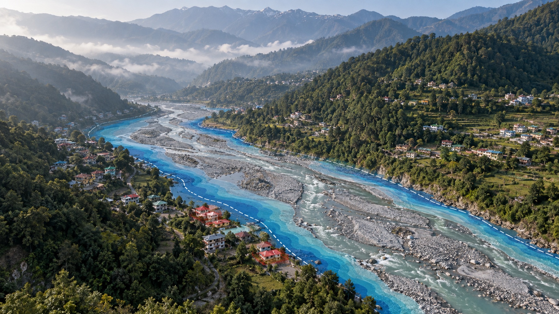
Conventional proximity analysis commonly assumes that the places nearer to a river are more exposed. In steep Himalayan terrain, straight line distance alone can be misleading: a building closer to aa channel may sit above it, while another building farther away from a channel may lie on a low, hydrologically connected surface. The project tests whether terrain-aware indicators improve the identification of potentially exposed buildings in the Maldevta flash floods.
River Buffer and HAND Exposure Analysis for the Maldevta Song Watershed
Building Exposure during the August 2022 flash flood, Song watershed above Doiwala Outlet, Dehradun, Uttarakhand- 457.5 km2
PROBLEM STATEMENT
The project tests whether terrain-aware indicators improve the identification of potentially exposed buildings in the Maldevta flash floods.
RESEARCH QUESTION
How much and where do simple river buffer and terrain-aware HAND methods disagree when identifying potentially exposed buildings during the 2022 Maldevta flash flood?
INTRODUCTION
A severe rainfall event affected the Maldevta-Song area during the night of 19 August and the early hours of 20 August 2022. Published studies describe damaged buildings, roads, bridges, farms and river banks around Maldevta, Sarkhet, Kumalda, Bhaiswar and Thano. The event showed that being close to a river is important, but distance alone does not explain where water can spread.
Conventional proximity analysis commonly assumes that the places nearer to a river are more exposed. In steep Himalayan terrain, straight line distance alone can be misleading: a building closer to aa channel may sit above it, while another building farther away from a channel may lie on a low, hydrologically connected surface.
This report compares two simple ways of screening building exposure. The first is a river buffer, which asks how close a building is to a channel. The second is Height Above Nearest Drainage, usually shortened to HAND, which asks how high the building stands above the stream reached by local drainage.
The analysis is a screening exercise. It helps identify places that deserve closer study, but it does not calculate flood depth, flow speed, damage or the probability of a future flood.
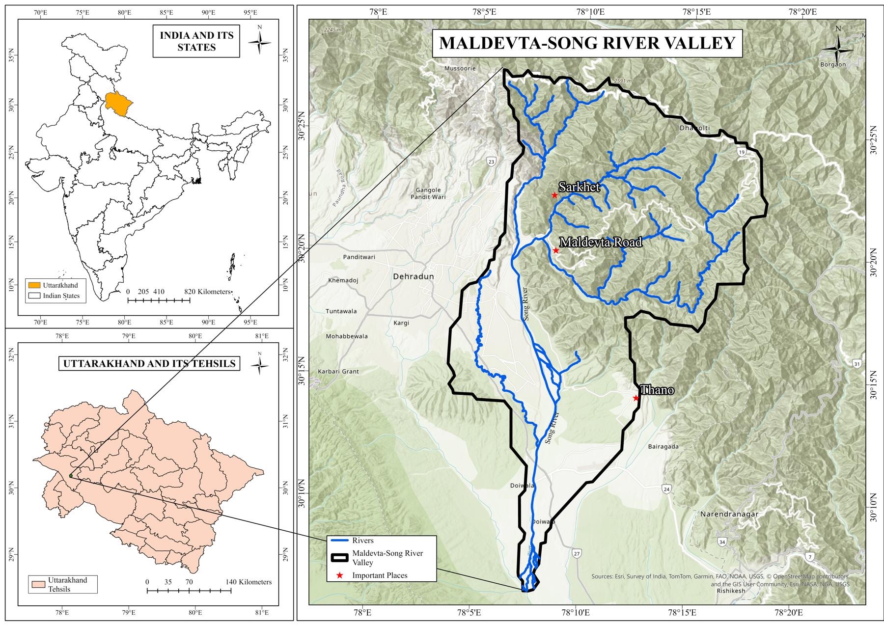
Figure 1. Location of the Maldevta-Song River Valley study area in Uttarakhand, with the watershed boundary and main mapped rivers.
Source: HydroBASINS boundary and OpenStreetMap river data.
Interpretation: The watershed follows the land that drains towards the selected outlet. It contains the Song main channel, western tributaries around Maldevta and Sarkhet, eastern headwaters and the lower valley towards Doiwala. Using a watershed is more meaningful than using a rectangular box because water follows slopes and channels, not map borders.
OBJECTIVES
- Describe the Maldevta-Song watershed and the data used in the study.
- Identify buildings close to modelled drainage channels using 50 m, 100 m and 250 m buffers.
- Identify buildings on low terrain using HAND thresholds of 3 m, 5 m and 10 m.
- Compare the buffer and HAND results and explain where they agree or disagree.
- Check whether the HAND result changes when different elevation models and channel thresholds are used.
DATA
All spatial layers were converted to WGS 1984 UTM Zone 44N, EPSG 32644. This projection measures distance in metres, which is necessary for reliable buffers, areas and channel calculations.
Table 1. Data used in the exposure analysis
| Dataset | Date or resolution | Use in the study |
|---|---|---|
| HydroBASINS Level 12 | Generalised global watershed data | Study-area boundary and outlet-based watershed |
| Google Open Buildings v3 | Building polygons; confidence at least 0.70 | Inventory of building footprints |
| SRTM GL1 | 30 m elevation grid | Primary terrain model |
| AW3D30 | 30 m elevation grid | Alternative terrain model for sensitivity testing |
| Copernicus GLO-30 | 30 m elevation grid | Alternative terrain model for sensitivity testing |
| OpenStreetMap | Historical state on 18 August 2022 | Mapped rivers and streams used as a reference |
| ESA WorldCover 2021 | 10 m land-cover map | Map background and landscape context only |
| Published event evidence | 56 records; 31 with coordinates | Independent check at reported damage locations |
Interpretation: The main building inventory contains 90,154 Google Open Buildings footprints inside the watershed. This is much larger than the earlier OpenStreetMap-only building set because Open Buildings uses satellite-image mapping over a wider area. The two inventories should not be mixed in one set of percentages.
- The study area covers 457.5 square kilometres and contains three connected HydroBASINS units.
- Elevation ranges from 282 m in the lower valley to 2,763 m near the Mussoorie ridge.
- A total of 90,390 building footprints were downloaded and 90,154 had their centre inside the watershed.
- The median building footprint area is 84 square metres.
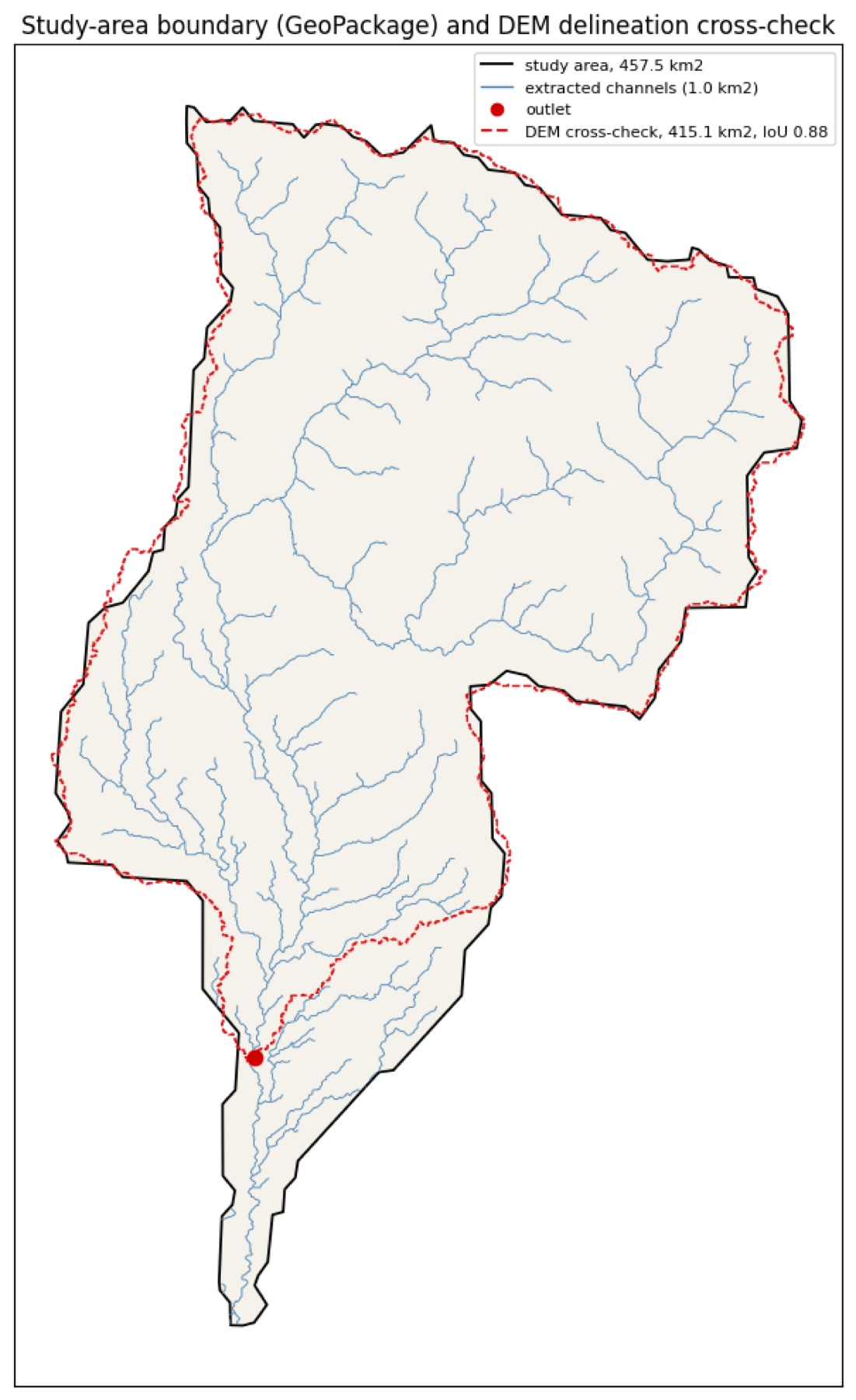
Figure 2. HydroBASINS study boundary compared with a watershed independently traced from the SRTM elevation model.
Source: project Figure 2; SRTM and HydroBASINS cross-check.
Interpretation: The black boundary covers 457.5 square kilometres. The red dashed boundary traced from the elevation model covers 415.1 square kilometres. Their intersection-over-union score is 0.88, where 1.00 would be a perfect match. The strong overlap supports use of the HydroBASINS boundary, while the difference near the southern end remains a limitation.
METHODS AND METHODOLOGY
The work followed the same sequence for every elevation model.
- Prepare the elevation models
Small artificial pits in an elevation grid can stop computer-modelled water. The elevation models were therefore conditioned by opening low-cost drainage paths through pits and filling only the depressions that remained.
- Calculate drainage direction and contributing area
Each 30 m cell was connected to the steepest of its eight neighbours. The model then counted the land area draining through every cell. Cells receiving water from a large area represent more important channels.
- Extract channels
A channel begins when its upstream contributing area reaches a chosen threshold. Three thresholds were tested: 0.5, 1.0 and 2.0 square kilometres. A smaller threshold creates many small tributaries; a larger threshold keeps only the larger streams.
Table 2. Extracted channel networks
| Elevation model | Threshold km2 | Length km | Density km per km2 |
|---|---|---|---|
| SRTM | 0.5 | 513.6 | 1.12 |
| SRTM | 1.0 | 372.4 | 0.81 |
| SRTM | 2.0 | 271.0 | 0.59 |
| AW3D30 | 0.5 | 531.0 | 1.16 |
| AW3D30 | 1.0 | 381.0 | 0.83 |
| AW3D30 | 2.0 | 281.0 | 0.61 |
| GLO-30 | 0.5 | 535.0 | 1.17 |
| GLO-30 | 1.0 | 380.1 | 0.83 |
| GLO-30 | 2.0 | 266.6 | 0.58 |
Interpretation. The 0.5 square kilometre threshold finds more of the mapped rivers but also creates many channels not present in OpenStreetMap. The 2.0 square kilometre threshold produces a simpler network but misses more mapped river length. The 1.0 square kilometre threshold was selected as the main compromise. OpenStreetMap is incomplete in small mountain valleys, so unmatched modelled channels are not automatically errors.
- Apply the buffer method
The centre of each building was measured in a straight line to the extracted channel network. A building was flagged when it fell within 50 m, 100 m or 250 m. These classes are cumulative: every building inside 50 m is also inside 100 m and 250 m.
- Calculate HAND
For each building, the model followed the drainage path downhill to the nearest channel and measured the elevation difference. A HAND value of 4 m means that the building stands about 4 m above the channel reached by that drainage path. It does not mean that 4 m of water will occur there.
HAND thresholds of 3 m, 5 m and 10 m were tested. The main comparison uses HAND below 5 m because reported flood depths during the event were approximately 3.5 to 5 m. This provides a practical screening threshold, not a direct flood-depth model.
- Compare the methods
Table 3. Meaning of the four comparison classes
| Class | Inside 100 m buffer | HAND below 5 m | Plain meaning |
|---|---|---|---|
| Both | Yes | Yes | Close to a channel and also on low terrain |
| Buffer only | Yes | No | Close to a channel but more elevated |
| Terrain only | No | Yes | Beyond 100 m but still on low connected terrain |
| Neither | No | No | Not flagged by either selected rule |
Agreement was summarised using the Jaccard index. This is the number of buildings flagged by both methods divided by the number flagged by either method. A score of 1 means complete agreement; a score of 0 means no shared buildings. Neither method was treated as the truth.
- Test sensitivity and stability
The HAND test was repeated for three elevation models and three channel thresholds, giving nine scenarios. Each building received a stability count from 0 to 9, showing how often it was classified below 5 m. This separates robust findings from buildings whose classification changes when the input model changes.
RESULTS
Overall exposure counts
Table 4. Buildings identified by the buffer and HAND methods
| Method | Class or threshold | Buildings | Share of 90,154 | How to read it |
|---|---|---|---|---|
| Buffer | Within 50 m | 8,621 | 9.6% | Immediate channel surroundings |
| Buffer | Within 100 m | 17,049 | 18.9% | Main buffer used for comparison |
| Buffer | Within 250 m | 40,627 | 45.1% | Broad distance screening |
| HAND | 0 to 3 m | 8,833 | 9.8% | Very low relative terrain |
| HAND | 3 to 5 m | 7,104 | 7.9% | Low relative terrain |
| HAND | 5 to 10 m | 17,383 | 19.3% | Moderately low terrain |
| HAND | 10 to 20 m | 25,727 | 28.5% | Higher above the channel |
| HAND | Above 20 m | 31,107 | 34.5% | Highest relative terrain class |
Interpretation. The 100 m buffer flags 17,049 buildings. HAND below 5 m flags 15,937 buildings, found by adding the 0 to 3 m and 3 to 5 m bands. The totals are similar, but similar totals do not mean that the same buildings were selected.
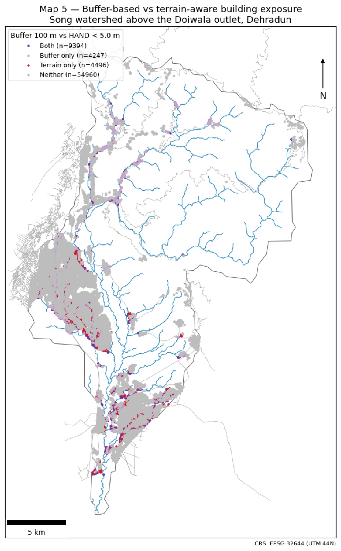
Figure 3. Comparison of the 100 m buffer and HAND below 5 m for the 90,154 building centroids
Interpretation: Purple points are identified by both methods. Light-purple points are close to a channel but stand higher than the 5 m HAND threshold. Red points are beyond the 100 m buffer but remain on low terrain connected to a channel. These red clusters show the main information added by HAND. Grey points are not flagged by either selected rule.
Main comparison
Table 5. 100 m buffer compared with HAND below 5 m for all buildings
| Class | Buildings | Share | Simple interpretation |
|---|---|---|---|
| Both | 10,902 | 12.1% | Both methods identify the building |
| Buffer only | 6,147 | 6.8% | Close to a channel, but higher terrain |
| Terrain only | 5,035 | 5.6% | Low terrain that lies beyond the buffer |
| Neither | 68,070 | 75.5% | Not identified by either selected threshold |
Interpretation: The methods disagree on 11,182 buildings: 6,147 are buffer only and 5,035 are terrain only. The Jaccard agreement is 0.494, meaning that the methods share only about half of the buildings identified by at least one method. Distance alone can over-classify elevated terraces and under-classify broad, low valley floors.
Sensitivity to the chosen thresholds
Table 6. Agreement under nine buffer and HAND threshold combinations
| Buffer m | HAND m | Both | Buffer only | Terrain only | Neither | Jaccard |
|---|---|---|---|---|---|---|
| 50 | 3 | 5,630 | 2,991 | 3,203 | 78,330 | 0.476 |
| 50 | 5 | 7,192 | 1,429 | 8,745 | 72,788 | 0.414 |
| 50 | 10 | 8,161 | 460 | 25,159 | 56,374 | 0.242 |
| 100 | 3 | 7,232 | 9,817 | 1,601 | 71,504 | 0.388 |
| 100 | 5 | 10,902 | 6,147 | 5,035 | 68,070 | 0.494 |
| 100 | 10 | 14,456 | 2,593 | 18,864 | 54,241 | 0.403 |
| 250 | 3 | 8,654 | 31,973 | 179 | 49,348 | 0.212 |
| 250 | 5 | 15,079 | 25,548 | 858 | 48,669 | 0.363 |
| 250 | 10 | 26,962 | 13,665 | 6,358 | 43,169 | 0.574 |
Interpretation: The amount of agreement changes when the thresholds change, but disagreement never disappears. Even the highest Jaccard score is 0.574. The terrain-only class is present in every combination, so the main finding is not caused by choosing only one convenient threshold pair.
Stability across elevation models
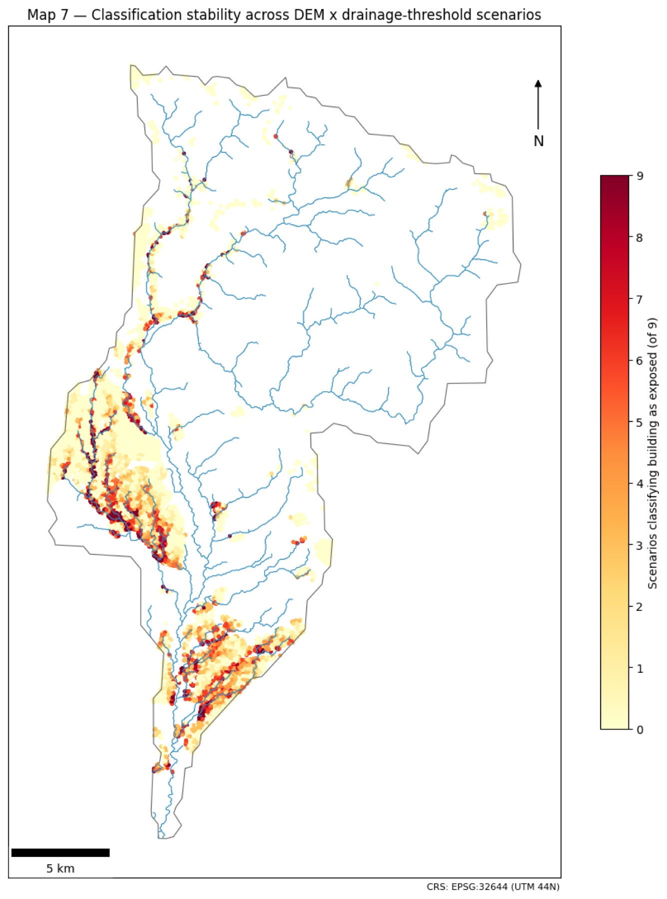
Figure 4. Number of the nine elevation-model and channel-threshold scenarios that classify each mapped building as below 5 m HAND.
Interpretation: Dark red buildings are repeatedly classified as low across many scenarios and are therefore the most stable part of the result. Pale yellow buildings are classified as low in few or no scenarios. The darkest clusters follow the main valley floors, while mixed colours around their edges show where small changes in the model alter the result.
Table 7. HAND exposure stability for all 90,154 buildings
| Stability class | Scenarios below 5 m | Buildings | Share | Meaning |
|---|---|---|---|---|
| Never flagged | 0 of 9 | 51,260 | 56.9% | Never classified below 5 m |
| Flagged occasionally | 1 to 3 of 9 | 21,812 | 24.2% | Occasionally classified below 5 m |
| Scenario-dependent | 4 to 6 of 9 | 11,212 | 12.4% | Result changes between scenarios |
| Flagged consistently | 7 to 9 of 9 | 5,870 | 6.5% | Usually classified below 5 m |
Interpretation: About 5,870 buildings are classified below 5 m in at least seven of the nine scenarios. This is the strongest and most repeatable exposure group. Buildings in the middle classes should be treated with more caution because their result depends on the elevation model or channel threshold.
Check against documented damage locations
Table 8. Selected evidence locations and the share of nearby buildings identified
| Location | Buildings nearby | Buffer 100 m | HAND below 5 m | Reading |
|---|---|---|---|---|
| Four Banyans resort | 14 | 100% | 100% | Both methods capture the site |
| Bandal-Song confluence | 44 | 100% | 100% | Both methods capture the site |
| Dhantu Sera | 16 | 81 to 100% | 62 to 77% | Both work, buffer captures more |
| Kumalda cluster | 208 | 88 to 97% | 57 to 70% | Both work, buffer captures more |
| Sarkhet | 67 | 72% | 4.5% | HAND misses most nearby buildings |
| Bhaiswar | 29 | 59% | 24% | Small tributary effects matter |
| Granny's Den | 2 | 100% | 0% | Close to channel but HAND above 5 m |
| Maldevta lower town | 393 | 0% | 0% | Modelled channel is offset in this reach |
Interpretation: Across 26 evidence rows with nearby buildings, the 100 m buffer identified an average of 61% of nearby buildings and HAND below 5 m identified 30%. Both methods worked well at several main-channel sites. HAND performed poorly at Sarkhet and Bhaiswar because damage there was linked to small steep tributaries below the main 1 square kilometre channel threshold. Both methods missed the listed Maldevta locations because the modelled channel was more than 100 m away from the mapped river in that wide braided reach.
Overall interpretation
The main conclusion is not that HAND is always better than a river buffer. The methods describe different parts of exposure. A buffer is simple and can capture buildings close to small mapped channels, but it ignores whether those buildings stand high above the watercourse. HAND includes terrain height and identifies low valley floors beyond a fixed buffer, but it can miss small tributary fans when those tributaries are absent from the modelled network.
For planning, the most sensible approach is to use both methods together. Buildings identified by both methods form a clear screening group. Buffer-only and terrain-only buildings show where local terrain, channel mapping and field information should be checked before decisions are made.
Limits on interpretation
- HAND is relative height above drainage, not predicted flood depth.
- The 30 m elevation cells are large compared with many narrow channels and buildings.
- SRTM, AW3D30 and GLO-30 are surface models; trees and roofs can raise measured elevations.
- Channels draining less than 1 square kilometre are missing from the primary network.
- The modelled channel is displaced from the mapped river in parts of the Maldevta braided reach.
- Google Open Buildings imagery does not have one exact 2022 acquisition date, so the inventory describes exposure rather than confirmed event damage.
- The evidence points are few, unevenly distributed and sometimes represent whole villages rather than exact buildings.
References
Dwivedi, S. K., Thakur, P. K., Dhote, P. R., Kruczkiewicz, A., Upadhyay, M., Moothedan, A. J., and Singh, R. P. (2024). Unravelling flash flood dynamics of Song watershed, Doon Valley: key insights for floodplain management. Geomatics, Natural Hazards and Risk, 15(1), 2378979. https://doi.org/10.1080/19475705.2024.2378979
European Space Agency. (2021). Copernicus DEM - Global and European Digital Elevation Model. https://doi.org/10.5270/ESA-c5d3d65
Jaccard, P. (1912). The distribution of the flora in the alpine zone. New Phytologist, 11(2), 37-50.
Khanduri, S. (2024). Cloudbursts strike over foothills Himalaya of Uttarakhand, India: a case study from Maldeota, Dehradun district. Academic Platform Journal of Natural Hazards and Disaster Management, 5(1), 30-45. https://doi.org/10.52114/apjhad.1434612
Lehner, B., and Grill, G. (2013). Global river hydrography and network routing: baseline data and new approaches to study the world's large river systems. Hydrological Processes, 27(15), 2171-2186.
Linke, S., Lehner, B., Ouellet Dallaire, C., and others. (2019). Global hydro-environmental sub-basin and river reach characteristics at high spatial resolution. Scientific Data, 6, 283.
Nobre, A. D., Cuartas, L. A., Hodnett, M., and others. (2011). Height Above the Nearest Drainage: a hydrologically relevant new terrain model. Journal of Hydrology, 404(1-2), 13-29.
Nobre, A. D., Cuartas, L. A., Momo, M. R., Severo, D. L., Pinheiro, A., and Nobre, C. A. (2016). HAND contour: a new proxy predictor of inundation extent. Hydrological Processes, 30(2), 320-333.
OpenStreetMap contributors. (2022). OpenStreetMap database, historical state of 18 August 2022, retrieved through the Overpass API. https://www.openstreetmap.org
Renno, C. D., Nobre, A. D., Cuartas, L. A., Soares, J. V., Hodnett, M. G., Tomasella, J., and Waterloo, M. J. (2008). HAND, a new terrain descriptor using SRTM-DEM. Remote Sensing of Environment, 112(9), 3469-3481.
Sain, K., Mehta, M., Kumar, V., Gupta, V., and Chauhan, P. (2023). A climatic surprise: slope instability triggered by heavy rain in Maldevta region, Dehradun, Uttarakhand, on 20 August 2022. Journal of the Geological Society of India, 99(3), 317-320. https://doi.org/10.1007/s12594-023-2313-1
Tadono, T., Ishida, H., Oda, F., Naito, S., Minakawa, K., and Iwamoto, H. (2014). Precise global DEM generation by ALOS PRISM. ISPRS Annals of the Photogrammetry, Remote Sensing and Spatial Information Sciences, II-4, 71-76.
Zanaga, D., Van De Kerchove, R., Daems, D., and others. (2022). ESA WorldCover 10 m 2021 v200. Zenodo. https://doi.org/10.5281/zenodo.7254221
Data attribution
- OpenStreetMap contributors (ODbL)
- Google Open Buildings v3 (CC BY 4.0 / ODbL)
- NASA SRTM (public domain)
- JAXA AW3D30 (JAXA terms)
- Copernicus DEM (Copernicus licence)
- ESA WorldCover 2021 (CC BY 4.0)
- HydroSHEDS and HydroBASINS (HydroSHEDS licence)