Check USGS Lidar Before Making a DEM in QGIS
A practical QGIS workflow for inspecting USGS 3DEP lidar over Hood River, Oregon, checking density and classification before deriving a bare-earth surface.
- Published
- Reading time
- 9 min
- Place
- Hood River Valley, Oregon, United States
- By
- Jannat Khosla
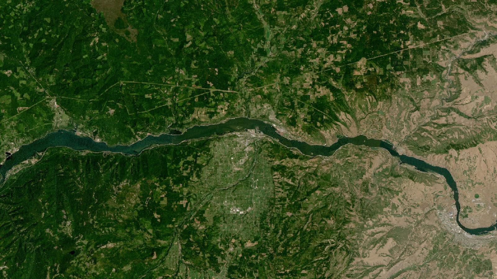
Cover: Landsat imagery of Hood River Valley, Oregon, United States, NASA (public domain).
Check the point cloud before you trust the surface
A lidar-derived elevation surface can look remarkably convincing while still being a poor input for drainage, slope or site-design work. That is especially easy to miss when working with ready-made rasters. A clean hillshade hides sparse strips, classification errors and gaps beneath vegetation. The safer starting point is the point cloud and its project metadata.
This walkthrough uses the Hood River valley in Oregon, United States, as a compact example. It is a useful setting because orchards, steep valley sides, roads and the Columbia River waterfront put several common lidar decisions in view. The method applies elsewhere in the United States where USGS 3D Elevation Program (3DEP) coverage is available.
USGS makes lidar point clouds and lidar-derived DEMs available through its elevation-focused LidarExplorer. The viewer supports an area-of-interest search and exposes project metadata, coverage, download sizes, lidar quality level and DEM-resolution availability, so it should be the first stop rather than a search for an anonymous DEM file. USGS GIS Data Download
The key habit is simple: decide what elevation represents before choosing a raster. A digital surface model describes the tops of features that intercept the sensor, such as trees and roofs. A bare-earth DEM attempts to represent terrain after non-ground features are removed. They answer different questions. A surface appropriate for checking canopy height can create invented ridges across a road corridor when used for flow routing.
Read the quality level as a specification, not a promise
3DEP quality levels combine a density or spacing requirement with a vertical-accuracy requirement. For lidar, USGS lists QL1 with a nominal pulse spacing of no more than 0.35 m, nominal pulse density of at least 8 points per square metre and 10 cm vertical RMSEz. QL2 has no more than 0.71 m spacing, at least 2 points per square metre and 10 cm vertical RMSEz. QL3 has no more than 1.41 m spacing, at least 0.5 points per square metre and 20 cm vertical RMSEz. USGS Topographic Data Quality Levels
Those figures describe collection requirements, not a licence to claim that every grid cell in a derived DEM is accurate to the same number. Terrain, vegetation, water, interpolation choices and point classification still matter. USGS itself notes that a greater pulse density can be needed depending on terrain and land cover. Its collection specification also identifies water, low near-infrared reflectivity surfaces and lidar shadowing as possible causes of data voids. USGS Lidar Base Specification, collection requirements
For a Hood River hillside, that distinction matters more than memorising the quality label. A QL2 dataset may be perfectly suitable for a broad erosion-screening map but still warrant local inspection before you set out a shallow drainage divide or report a small cut-and-fill estimate.
The other metadata fields deserve equal attention. Record the project name, acquisition date, horizontal and vertical coordinate reference systems, vertical datum, units, quality level and whether the download is source point cloud or an already-derived elevation raster. Keep this information in the QGIS project notes or a small text file alongside the source data. It makes an analysis reproducible and prevents a familiar later problem, where a good-looking layer cannot be explained or compared.
Worked example: a ground-density check in QGIS
The aim here is not to produce a polished terrain map immediately. It is to establish whether the downloaded points support the proposed terrain task and to identify where the answer needs caution.
1. Select a small area and download deliberately
Open USGS LidarExplorer and draw an area around the Hood River reach or a particular hillside. Review the returned project information before downloading. Download a small point-cloud subset for the first pass, rather than a large county-wide archive. USGS lists LAS and LAZ as formats for lidar point clouds, while its elevation downloads include several raster products. USGS elevation datasets and formats
A small subset gives you a quick way to inspect classifications and density without letting file size dictate the rest of the work. Return to the full extent only after the pilot area behaves as expected.
2. Load the point cloud and inspect its attributes
Add the LAS or LAZ file to QGIS. Open the layer properties and inspect available dimensions or attributes. QGIS selects an RGB renderer when colour attributes are present; otherwise it uses Classification when that attribute exists, then falls back to elevation, labelled Z. The Statistics tab is useful for seeing which attributes are present and their ranges. QGIS point-cloud documentation
Start with Classification rendering if it is available. Pan across orchard blocks, roads and wooded ground. You are looking for plausibility, not perfection: do ground points broadly follow the visible terrain? Do elevated points occur where tree crowns or buildings should be? Are there broad blank patches or seams that may affect a derived surface?
Switch to Z rendering briefly as a second visual check. Colouring by elevation can reveal sudden steps between flight strips or suspiciously flat areas. It will not prove an error, but it tells you where to inspect more closely.
3. Make a density raster, then make it meaningful
Open Processing and run Point cloud extraction > Density. QGIS documents this tool as exporting a raster based on the number of points in each raster cell for quality checking. It allows a chosen output resolution and an optional PDAL filter expression or crop extent. QGIS Point Cloud Extraction
For the first run, use all points and choose a cell size that lets you see local changes without producing a visually noisy raster. Style the result with a single-hue ramp where low counts are conspicuous. Compare it with an aerial basemap and the point-cloud view. Water, dark roofs and steep faces may legitimately have low returns, but an unexplained low-density strip crossing ordinary land deserves a note.
Then repeat the density calculation with a filter expression that selects the ground classification available in the file. Do not assume the existing classification is correct merely because it has a ground label. Compare the filtered view with the unfiltered cloud along roads, orchard rows and forest edges. The difference between all-return density and ground-return density is often the useful diagnostic. A high-density canopy does not mean a high-confidence bare-earth terrain model beneath it.
4. Extract a local review subset
Use Point cloud extraction > Filter to crop the most consequential part of the site, such as a proposed drainage crossing or a steep road approach. QGIS can filter by a PDAL expression, a cropping rectangle, or both, and can write LAS, LAZ, COPC.LAZ or VPC output. QGIS Point Cloud Extraction
Work with that local copy in QGIS’s 3D view. Rotate it so that a slope is seen obliquely, not only from above. Misclassified vegetation and a gap beneath a dense stand are much easier to recognise in this view. Record any exclusion areas before you create contours, calculate slope or derive flow paths.
5. Derive and validate the terrain product
If the point cloud’s supplied ground classification passes the visual and density checks, use a ground-only subset as the basis for a DEM. Use a projected coordinate reference system with metre units for a local Hood River analysis, and retain the source vertical datum in the output metadata. Pick a grid resolution that fits the data quality and decision scale. A finer grid is an interpolation choice, not evidence that the terrain has gained detail.
Overlay hillshade, contours and a semi-transparent aerial image. Follow several known road edges, channel margins and open fields. If field data, engineering survey points or a suitably documented local reference layer exist, use them as independent checks. Do not validate a terrain model by comparing it only with a hillshade made from the same model.
The beginner mistake: treating a downloaded DEM as ground truth
The costly mistake is assuming that the smallest available pixel is automatically the most reliable answer. Pixel size, point density, vertical accuracy, acquisition conditions and classification quality are separate properties. A 1 m raster derived from sparse or badly classified ground points can look precise while placing a drainage crest or roadside ditch in the wrong position.
Avoid this by writing a short fitness statement before analysis. For example: “This 3DEP dataset is being used to screen broad drainage patterns near Hood River; areas with low ground-point density or obvious canopy effects will not support parcel-scale design measurements.” This makes the limitation visible to the next analyst and keeps map symbology from overstating certainty.
USGS requires conventional 3DEP lidar collection to deliver multiple discrete returns, with data collection capable of at least three returns per pulse. That improves the opportunity to observe through vegetation, but it does not guarantee a clean ground return at every location. USGS Lidar Base Specification, collection requirements
There is a second mistake worth avoiding: silently mixing elevation sources. A project can contain lidar-derived terrain, imagery-derived elevation and other products with different properties. Name layers clearly, preserve source metadata, and do not mosaic datasets until their datums, dates and intended roles have been checked.
Frequently asked questions
Is QL2 lidar adequate for a Hood River drainage-screening map?
Yes, QL2 can support a broad drainage-screening map when its local ground-point coverage and classification are checked first. USGS defines QL2 using at least 2 points per square metre, no more than 0.71 m nominal pulse spacing and 10 cm vertical RMSEz, but site conditions still govern suitability.
Should I use all lidar returns to make a bare-earth DEM?
No, a bare-earth DEM should be based on ground points or a documented ground-classification process. All returns include vegetation and built features, which can distort slope, contours and flow paths. Inspect the point cloud before trusting an existing ground classification.
Can QGIS inspect LAS and LAZ point clouds directly?
Yes, QGIS can load point-cloud data and render it by RGB, classification or elevation attributes. Its point-cloud extraction tools can create density rasters and filtered LAS, LAZ, COPC.LAZ or VPC subsets, subject to the documented PDAL requirement.
Why does my density raster show gaps over water and roofs?
Those gaps can be real acquisition effects, because water, low near-infrared reflectivity surfaces and lidar shadowing can produce data voids. Treat them as areas requiring interpretation rather than automatically filling them with interpolated terrain values.
References
- USGS, GIS Data Download and LidarExplorer
- USGS, Topographic Data Quality Levels
- USGS, Lidar Base Specification: Collection Requirements
- USGS, elevation datasets, formats and downloads
- QGIS documentation, Working with Point Clouds
- QGIS documentation, Point Cloud Extraction
Researched and drafted with AI assistance; sources are linked for verification.
Need this done for your own study area? Send me the area and what you need.
Cite this post
Khosla, J. (2026, November 11). Check USGS Lidar Before Making a DEM in QGIS. Jannat Khosla. https://jannatkhosla.com/blog/check-usgs-lidar-before-making-a-dem-in-qgis
› BibTeX
@online{khosla2026check,
  author = {Khosla, Jannat},
  title = {Check USGS Lidar Before Making a DEM in QGIS},
  date = {2026-11-11},
  url = {https://jannatkhosla.com/blog/check-usgs-lidar-before-making-a-dem-in-qgis}
}