Estimating Crop Yield with SAR and Optical Data Fusion in GEE
Cloud cover during India's kharif season makes optical-only yield models unreliable. This article shows how to fuse Sentinel-1 SAR and Sentinel-2 data in Google Earth Engine to build a cloud-robust crop yield estimation workflow.
Why Single-Sensor Approaches Fall Short in India's Cropping Calendar
India's two dominant cropping seasons, kharif (June–November) and rabi (November–April), present a fundamental remote sensing challenge: the kharif season coincides almost exactly with the southwest monsoon. Cloud cover during June through September routinely renders optical imagery unusable for weeks at a stretch, precisely when crops are establishing and reaching peak vegetative growth. If you are building a crop yield estimation remote sensing workflow that relies only on Sentinel-2 or Landsat, you will have data gaps exactly where the phenological signal matters most.
This is not a minor inconvenience. Missing the vegetative peak of a paddy or soybean crop means your time-series indices - NDVI, EVI, LAI proxies, are truncated. A truncated time series produces unreliable yield forecasts. The practical fix that has gained traction in recent years is fusing Sentinel-1 SAR (Synthetic Aperture Radar) with Sentinel-2 optical data inside Google Earth Engine (GEE), exploiting the fact that SAR sees through clouds by design.
What Each Sensor Actually Contributes
Before fusing anything, it helps to be precise about what each sensor measures and why that matters for yield.
Sentinel-2 (optical, 10–20 m):
- Reflectance in red, NIR, and SWIR bands supports vegetation indices like NDVI, EVI, and the red-edge chlorophyll index (CIre).
- These indices correlate with green leaf area and chlorophyll content, both proxies for photosynthetic capacity and, ultimately, biomass accumulation.
- Limitation: cloud masking with the Scene Classification Layer (SCL) removes large portions of kharif imagery.
Sentinel-1 (C-band SAR, 10 m, VV and VH polarisations):
- Backscatter in VH polarisation is sensitive to vegetation volume and canopy structure. For rice in particular, VH backscatter rises steeply during tillering and heading, then drops after senescence, a well-documented phenological signature.
- VV polarisation responds more to surface roughness and soil moisture, useful for detecting bare soil between cropping cycles.
- Limitation: SAR backscatter is influenced by wind-induced canopy motion, incidence angle variation, and speckle noise. It does not directly measure chlorophyll.
The fusion logic is straightforward: SAR fills the temporal gaps in optical coverage during monsoon months; optical data anchors the chlorophyll and greenness signal during clear periods. Together they produce a denser, more complete time series across the entire crop season.
Setting Up the Fusion Workflow in GEE
Here is a practical outline of how to structure this in GEE for a kharif paddy district, say, West Godavari in Andhra Pradesh or Chhattisgarh's rice bowl.
Step 1 - Define your region and season
Draw or import a district boundary as a FeatureCollection. Set the date range to cover sowing through harvest, typically 1 June to 30 November for kharif paddy.
Step 2 - Build the Sentinel-2 time series
Filter COPERNICUS/S2_SR_HARMONIZED by region and date. Apply the SCL-based cloud mask (keep classes 4 and 5, vegetation and bare soil). Compute NDVI and the red-edge index (CIre = (NIR / Red-edge) − 1) for each image. Reduce to a monthly or dekadal (10-day) composite using .median().
Step 3 - Build the Sentinel-1 time series
Filter COPERNICUS/S1_GRD for IW mode, VV+VH polarisation, and descending orbit (more consistent geometry over most Indian districts). Apply a refined Lee speckle filter - GEE does not include one natively, but community scripts are available. Compute the VH/VV ratio, which partially normalises for soil moisture effects. Reduce to the same dekadal composites.
Step 4 - Merge into a single multi-band image collection
Join the two collections on date using ee.Join.saveFirst() with a temporal tolerance of ±5 days. Stack SAR and optical bands into one image per time step. You now have a cloud-robust time series with both structural (SAR) and biochemical (optical) information.
Step 5 - Extract features for yield modelling
For each field polygon (or a grid of pixels), extract:
- Maximum NDVI and the date it occurs (heading date proxy)
- Cumulative VH backscatter integral over the season (related to total canopy development)
- NDVI–VH correlation coefficient (a crop-type discriminator)
- Length of the green period above an NDVI threshold
These features feed into a regression model - Random Forest works well here because it handles the non-linear interactions between SAR and optical features without requiring normalisation.
Step 6 - Calibrate against reported yield data
Use district-level yield statistics from the Directorate of Economics and Statistics (DES), Ministry of Agriculture & Farmers Welfare, or crop-cutting experiment data where available. Split by year for temporal cross-validation rather than random split, since yield data has inter-annual autocorrelation.
Why the Red-Edge Bands Matter More Than NDVI Alone
A common mistake in crop yield estimation remote sensing projects is stopping at NDVI. NDVI saturates at moderate-to-high canopy densities, exactly the conditions you encounter in irrigated paddy fields at peak growth. Sentinel-2's red-edge bands (B5 at 705 nm, B6 at 740 nm, B7 at 783 nm) remain sensitive at higher LAI values because chlorophyll absorption at these wavelengths does not saturate as quickly.
For rabi wheat in Punjab or Haryana, where fields are dense and relatively cloud-free, adding CIre alongside NDVI consistently improves model fit. The red-edge also helps distinguish stressed crops (lower chlorophyll, lower CIre) from healthy ones at similar NDVI levels, a distinction that matters when you are trying to explain yield variability within a district, not just between districts.
Handling the Rabi Season Differently
Rabi crops (wheat, mustard, chickpea) grow during the dry, cool months when cloud cover is minimal across most of India. Here, the SAR contribution shifts: rather than filling cloud gaps, Sentinel-1 helps distinguish crop types that look spectrally similar in optical data. Mustard and wheat have overlapping NDVI trajectories in December–January, but their canopy structures differ enough that VH backscatter time series separate them reliably.
For rabi yield forecasting, a practical approach is to use optical data as the primary signal (given clear skies) and SAR as a crop-type mask to ensure you are not mixing mustard and wheat pixels in your wheat yield model. Running a simple SAR-based classifier first, then applying crop-specific yield models, reduces within-district error substantially.
Limitations to Be Honest About
- Field boundary data: GEE gives you pixels; yield models need field boundaries. Without accurate cadastral or farmer-reported boundaries, you are aggregating over mixed pixels. The Bhuvan portal and some state governments provide parcel data, but coverage is uneven.
- Crop-cutting experiment gaps: DES yield statistics are district averages derived from crop-cutting experiments that have known sampling limitations. Calibrating a pixel-level model against district averages introduces a scale mismatch.
- SAR incidence angle variation: Sentinel-1's repeat cycle and orbit geometry mean that backscatter values for the same crop can vary with incidence angle. Normalising by local incidence angle or restricting to a single relative orbit reduces this noise.
- Transplanting date variability: In paddy systems, transplanting dates shift by weeks depending on monsoon onset and water availability. A fixed phenological window will misalign for some districts in some years. Using dynamic thresholds (e.g., detect the onset of VH rise rather than using calendar dates) is more robust.
A Note on Scaling This Up
The workflow described here is tractable for a single district in GEE's free tier. Scaling to all paddy districts in India, roughly 150–200 districts that account for the bulk of production, requires either GEE Cloud Projects with higher compute quotas or exporting intermediate composites to Google Cloud Storage and running the regression offline. The export bottleneck is usually the SAR speckle filtering, which is computationally expensive at scale.
For national-scale operational systems, agencies like the Mahalanobis National Crop Forecast Centre (MNCFC) under the Ministry of Agriculture already run satellite-based crop area and yield estimation programmes. Understanding their methodology, which increasingly incorporates SAR, is useful context if you are building something that needs to interface with or validate against official forecasts.
Frequently asked questions
Why fuse SAR and optical data for crop yield estimation instead of using Sentinel-2 alone in India?
Because monsoon cloud cover during June–September routinely makes optical Sentinel-2 imagery unusable for weeks, exactly when kharif crops are establishing and hitting peak vegetative growth. Sentinel-1 SAR sees through clouds and fills those gaps, while optical data anchors the chlorophyll signal.
Which Sentinel-1 polarisation best tracks rice crop growth stages?
VH polarisation, which is sensitive to vegetation volume and canopy structure. For rice specifically, VH backscatter rises steeply during tillering and heading, then drops after senescence, a well-documented phenological signature used to track crop growth stages.
Why use Sentinel-2's red-edge bands instead of just NDVI for crop yield models?
NDVI saturates at moderate-to-high canopy densities, exactly the conditions in peak-growth irrigated paddy. Sentinel-2's red-edge bands (B5, B6, B7) stay sensitive at higher leaf area because chlorophyll absorption at those wavelengths doesn't saturate as quickly, helping separate stressed from healthy crops.
What yield data can I calibrate a GEE-based crop yield model against in India?
District-level yield statistics from the Directorate of Economics and Statistics (DES) under the Ministry of Agriculture & Farmers Welfare, or crop-cutting experiment data where available. Split the calibration by year rather than randomly, since yield data has inter-annual autocorrelation.
References
- Sentinel-1 mission overview: https://sentinel.esa.int/web/sentinel/missions/sentinel-1
- Sentinel-2 mission overview: https://sentinel.esa.int/web/sentinel/missions/sentinel-2
- Google Earth Engine data catalog - Sentinel-1 GRD: https://developers.google.com/earth-engine/datasets/catalog/COPERNICUS_S1_GRD
- Google Earth Engine data catalog - Sentinel-2 SR Harmonized: https://developers.google.com/earth-engine/datasets/catalog/COPERNICUS_S2_SR_HARMONIZED
- Mahalanobis National Crop Forecast Centre (MNCFC): https://www.mncfc.nic.in
- Directorate of Economics and Statistics, MoAFW: https://eands.dacnet.nic.in
Researched and drafted with AI assistance.
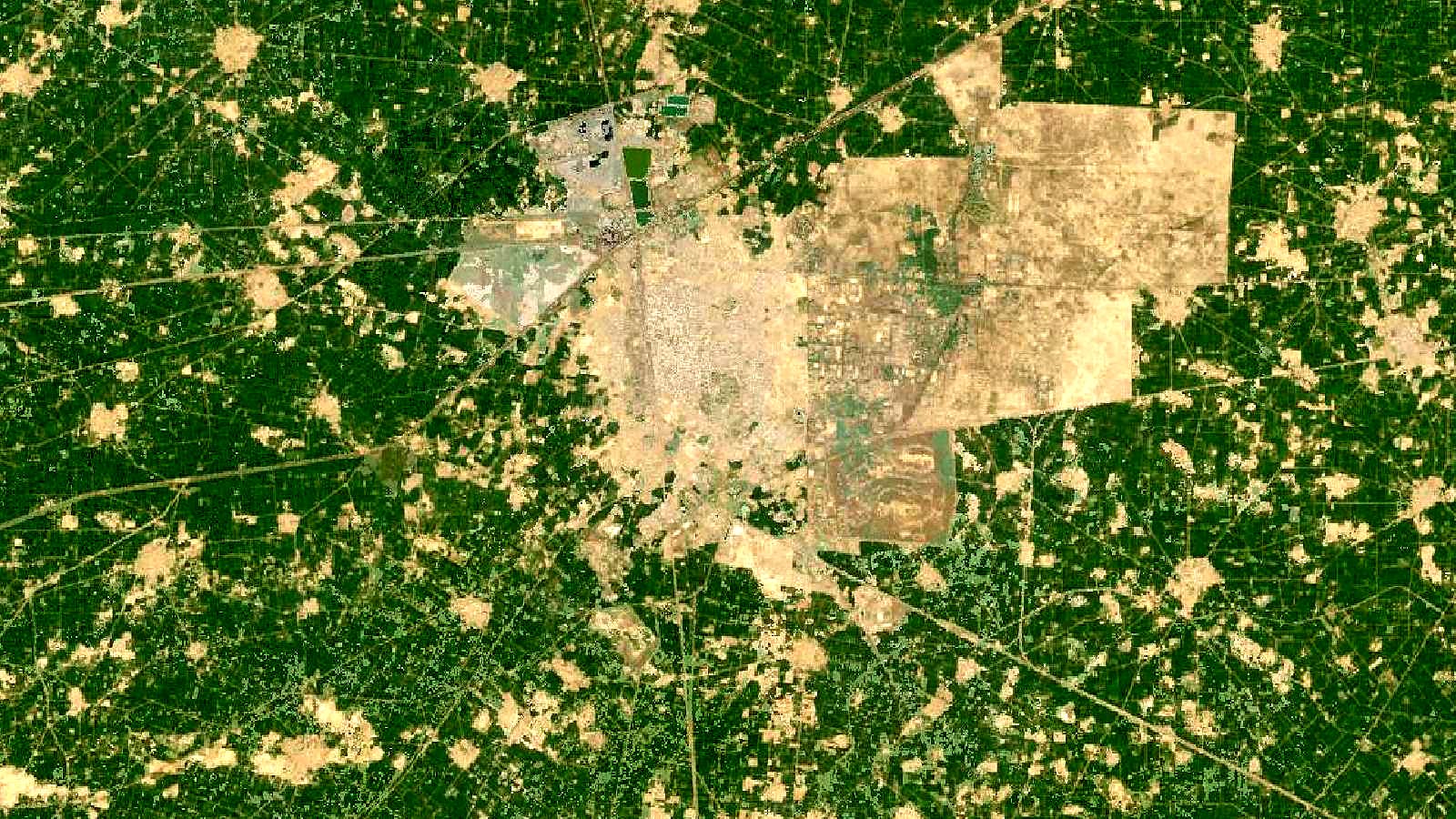
Cover image: Landsat true-colour composite of farmland near Bathinda, Punjab (2000), NASA/USGS Landsat WELD via NASA GIBS (public domain).