Flow Accumulation and Stream Order from DEM in QGIS: Step by Step
A step-by-step QGIS walkthrough of flow accumulation and stream ordering from a DEM, covering sink filling, flow direction, and common mistakes that silently break watershed delineation in Indian study areas.
Why the Middle Steps Keep Tripping People Up
Watershed delineation tutorials are everywhere. Type the phrase into any GIS forum and you will find a dozen walkthroughs, each one starting with a DEM and ending with a polygon. What those tutorials gloss over is the chain of preprocessing steps that sits between the raw elevation data and the final boundary, filling sinks, computing flow direction, accumulating flow, and ordering streams. Get any one of these wrong and your watershed polygon is quietly, invisibly incorrect. I have seen this happen repeatedly in student projects and in professional flood-risk reports alike.
This post works through each step in QGIS, explains what can go wrong, and shows you how to interpret the outputs before you move on to delineation.
What Data Do You Need Before You Start?
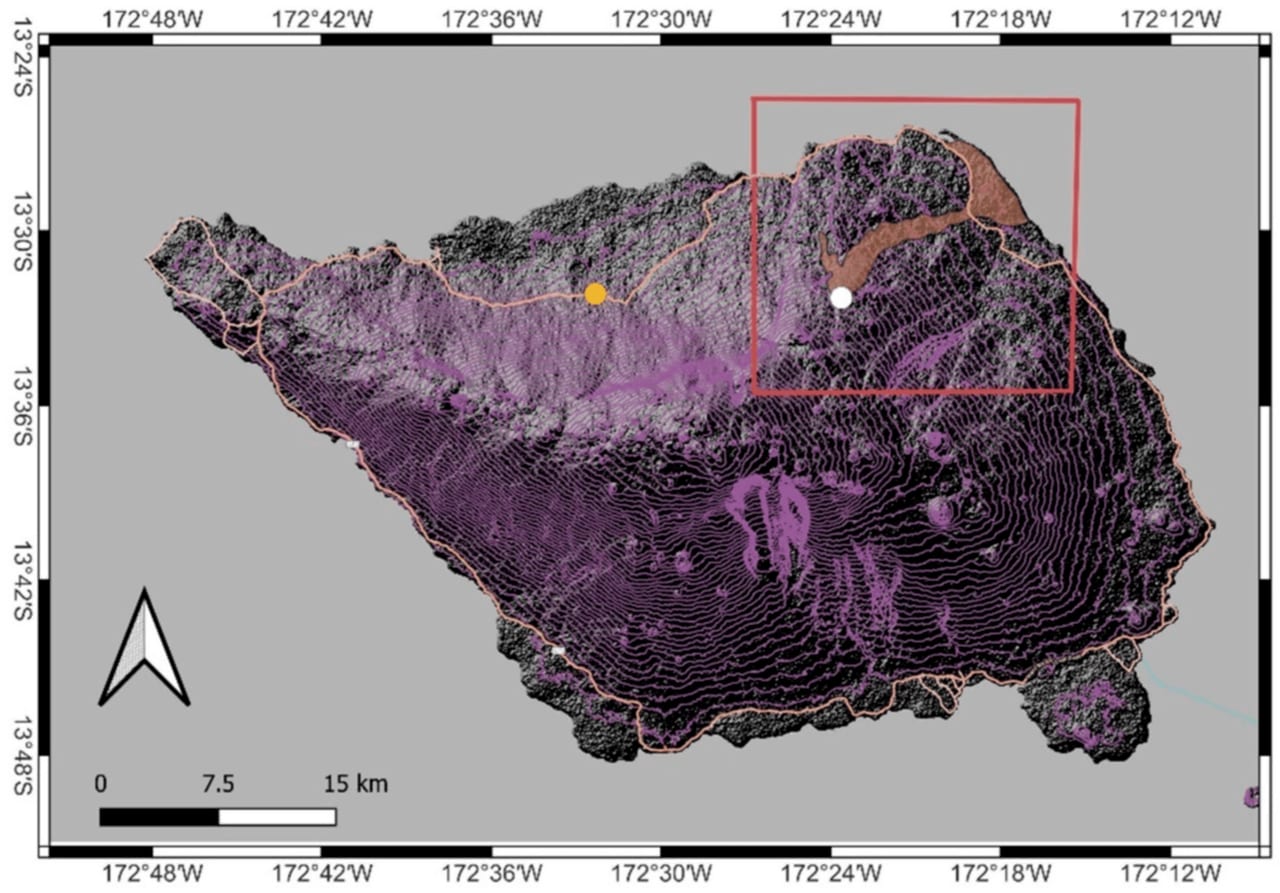
Illustrative: SRTM DEM hillshade river basin. "Proceedings-87-00033-g001" by Németh, K. (2022) is licensed under CC BY 4.0. To view a copy of this license, visit https://creativecommons.org/licenses/by/4.0/.
You need a Digital Elevation Model (DEM) in a projected coordinate reference system, not geographic (degrees). For most of India, UTM Zone 43N or 44N (WGS 84) is appropriate depending on your study area. Working in degrees will produce distorted flow directions because the raster cells are not square on the ground.
Good free DEM sources for Indian study areas:
- SRTM 30 m, adequate for basin-scale work, available from USGS EarthExplorer
- ALOS PALSAR 12.5 m, better for hilly terrain, available from ASF DAAC
- Cartosat-1 DEM (CartoDEM v3), ISRO's national product, ~30 m, available through Bhuvan
Download a tile that generously covers your study area. Clipping too tightly before processing causes edge artifacts in flow direction and accumulation.
Step 1 - Fill Sinks (and Why You Cannot Skip This)
A raw DEM contains sinks: cells or groups of cells where elevation is artificially lower than all neighbours. Some are real (a dry lake bed, a quarry), but most are interpolation artefacts. If you compute flow direction on an unfilled DEM, flow terminates at these sinks instead of routing to the outlet. Your accumulation grid will look like a leopard print, patches of high accumulation surrounded by dead zones.
In QGIS: Use the SAGA → Preprocessing → Fill Sinks (Wang & Liu) algorithm. It is more robust than the simpler Planchon-Darboux fill for Indian terrain, which often includes both flat agricultural plains and steep Himalayan or Western Ghats slopes in the same basin.
Key parameter: Minimum Slope, set it to a very small positive value (0.01 degrees is a common default). This prevents the algorithm from creating perfectly flat filled areas, which would cause undefined flow directions downstream.
Check your output: Subtract the original DEM from the filled DEM (Raster Calculator). Cells where the difference is greater than zero are filled sinks. If you see large contiguous patches of fill, say, several square kilometres, investigate whether those are real water bodies that should be masked out before processing.
Step 2 - Flow Direction
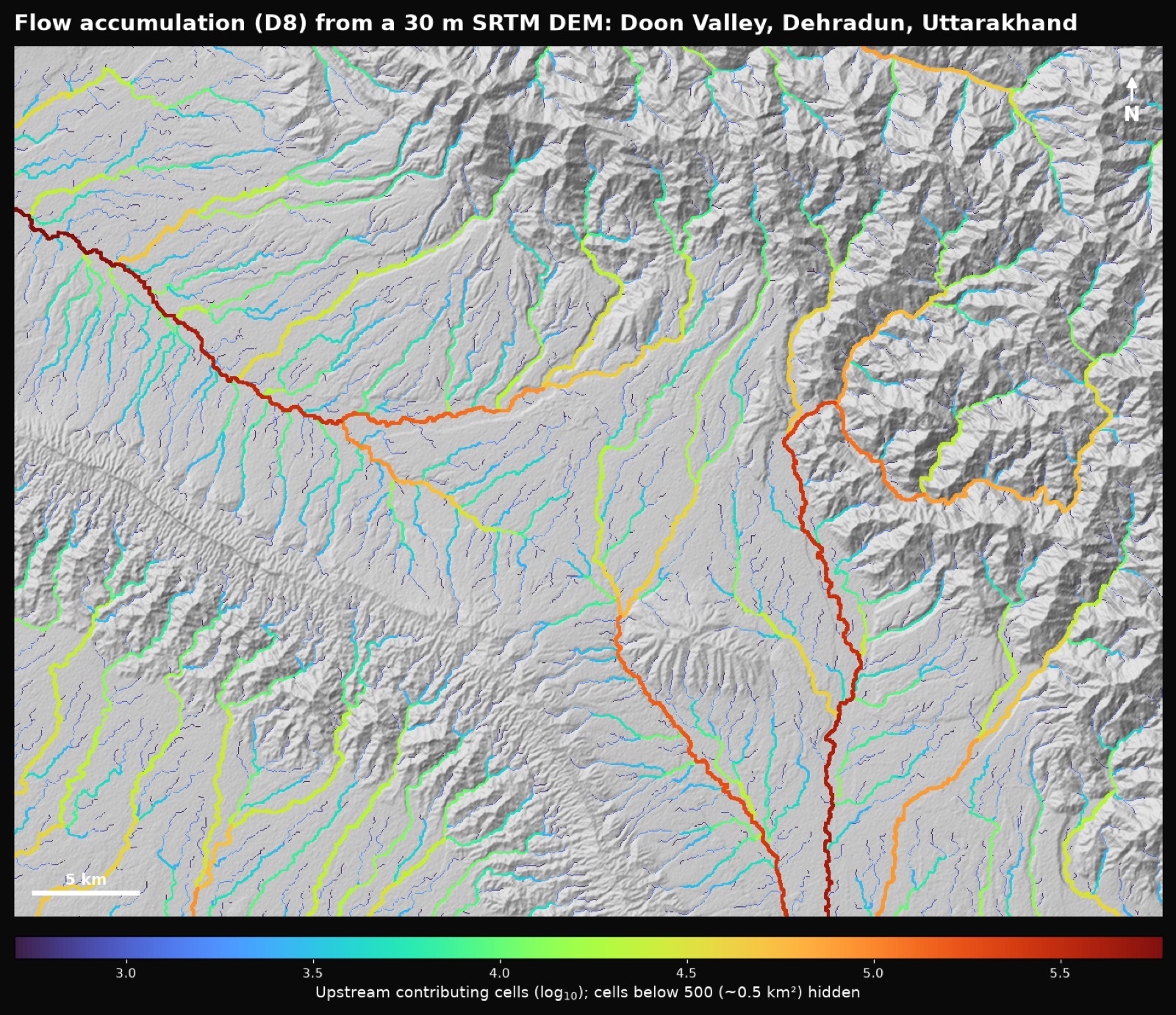
Flow accumulation (D8) computed from a 30 m SRTM DEM for the Doon Valley, Dehradun: channels are coloured by upstream contributing area on a log scale, and hillslope cells draining less than about 0.5 km² are hidden. Elevation data: AWS Terrain Tiles (Mapzen/Tilezen), SRTM courtesy NASA/USGS.
Flow direction assigns each cell a code indicating which of its eight neighbours it drains into (the D8 method). In SAGA this is called Flow Direction (D8) under Terrain Analysis → Preprocessing.
Common mistakes here:
- Running flow direction on the unfilled DEM (see Step 1)
- Using a DEM still in geographic coordinates, the algorithm will run without error but the results will be wrong
- Not checking for flat areas: large irrigated plains in Punjab or the Gangetic belt can produce large flat regions even after sink filling, and flow direction across them is unreliable without additional preprocessing
For flat areas, SAGA's Fill Sinks (Wang & Liu) with a non-zero minimum slope largely handles this. If you still see large flat zones, consider the Flow Direction (Rho8) algorithm which introduces a small stochastic component to break ties.
Step 3 - Flow Accumulation
Flow accumulation counts, for each cell, how many upstream cells drain into it. Cells with high accumulation values sit in valleys and channels; cells with low values are on ridges and hillslopes.
In QGIS: Run SAGA → Terrain Analysis → Flow Accumulation (Top-Down). Input is your flow direction raster.
The output values range from 1 (a hilltop cell with no upstream area) to potentially millions (a cell near a major river outlet). Visualise it with a logarithmic colour ramp, the default linear stretch will make everything look flat because the distribution is heavily skewed.
A simple worked example: Suppose your DEM has 10 m cells and a cell shows a flow accumulation value of 50,000. That cell drains approximately 50,000 × (10 × 10) = 5,000,000 m² = 5 km² of upstream area. This is a quick sanity check, compare it against known catchment areas from CWC gauging stations or published basin atlases.
Step 4 - Extracting a Stream Network
To convert the accumulation raster into a stream network, you apply a threshold: cells above a certain accumulation value are classified as streams.
In QGIS Raster Calculator:
"flow_accumulation@1" > 1000
This creates a binary raster, 1 where streams exist, 0 elsewhere. The threshold is the single most consequential decision in this step. A threshold that is too low produces a dense, noisy network with streams on every hillslope. Too high and you miss headwater tributaries.
There is no universal correct value. For a 30 m SRTM DEM in a semi-arid Indian watershed, a threshold equivalent to roughly 0.5–1 km² of upstream area is a reasonable starting point. Convert that to cells: 0.5 km² ÷ (30 m × 30 m) ≈ 556 cells. Adjust by comparing your extracted network against Survey of India topographic sheets or Bhuvan's drainage layers.
Step 5 - Strahler Stream Order
Strahler ordering assigns integer values to stream segments based on tributary hierarchy. Two first-order streams merge to form a second-order stream; two second-order streams form a third-order stream, and so on. It is the standard classification used in Indian hydrology reports and is required input for many geomorphometric analyses.
In QGIS: Use SAGA → Terrain Analysis → Strahler Order. The input is your flow direction raster (not the stream network raster - SAGA derives the network internally using the direction grid).
Interpreting the output:
| Strahler Order | Typical Meaning |
|---|---|
| 1 | Headwater channels, often seasonal in peninsular India |
| 2–3 | Minor perennial tributaries |
| 4–5 | Sub-basin scale rivers |
| 6+ | Major river trunks (Ganga, Godavari, Krishna mainstems) |
A basin with a maximum order of 4 or 5 is typical for a medium-sized Indian sub-watershed of a few hundred to a few thousand km².
Validating Your Results Before Moving to Delineation
Before you delineate a watershed, run these three checks:
- Visual overlay - Load your Strahler order raster or extracted stream network over a Google Satellite basemap (via XYZ tiles in QGIS). Do the channels follow visible valleys? Do they align with actual river courses?
- Outlet location - Snap your pour point to a high-accumulation cell. If the pour point falls on a low-accumulation cell, your watershed will be tiny or nonsensical.
- Area sanity check - Use the accumulation value at the outlet cell to estimate upstream area (cells × cell area). Compare against published basin areas from CWC, NRSC, or state water resource departments.
These three steps take ten minutes and will catch the majority of errors before you invest time in downstream analysis.
Frequently asked questions
Why do I need to fill sinks in a DEM before computing flow direction?
Because unfilled sinks, mostly interpolation artefacts, cause flow to terminate instead of routing to the outlet, leaving a patchy accumulation grid with high-accumulation cells surrounded by dead zones. Filling sinks first (e.g. SAGA's Wang & Liu algorithm) avoids this.
Which free DEM should I use for watershed delineation in India?
SRTM 30 m works for basin-scale mapping, ALOS PALSAR 12.5 m suits hilly terrain, and ISRO's Cartosat-1 CartoDEM (~30 m) is available via Bhuvan. Whichever you choose, reproject it to a projected CRS like UTM Zone 43N or 44N, not geographic degrees.
What flow accumulation threshold should I use to extract streams from a 30 m SRTM DEM?
For a 30 m SRTM DEM in a semi-arid Indian watershed, a threshold around 0.5–1 km² of upstream area (roughly 556 cells) is a reasonable starting point, adjusted by comparing the extracted network against Survey of India sheets or Bhuvan's drainage layers.
What does a Strahler stream order of 6 or higher represent?
A Strahler order of 6 or higher marks major river trunks, such as the Ganga, Godavari, or Krishna mainstems. Order 1 covers headwater channels, often seasonal in peninsular India, while orders 4–5 are typical for a medium-sized Indian sub-watershed.
References
- USGS EarthExplorer (SRTM data): https://earthexplorer.usgs.gov
- ASF DAAC (ALOS PALSAR DEM): https://asf.alaska.edu
- ISRO Bhuvan (CartoDEM, drainage layers): https://bhuvan.nrsc.gov.in
- QGIS Documentation: https://docs.qgis.org
- SAGA GIS Documentation: https://saga-gis.sourceforge.io/saga_tool_doc
- Central Water Commission, India (basin data reference): https://cwc.gov.in
Researched and drafted with AI assistance.
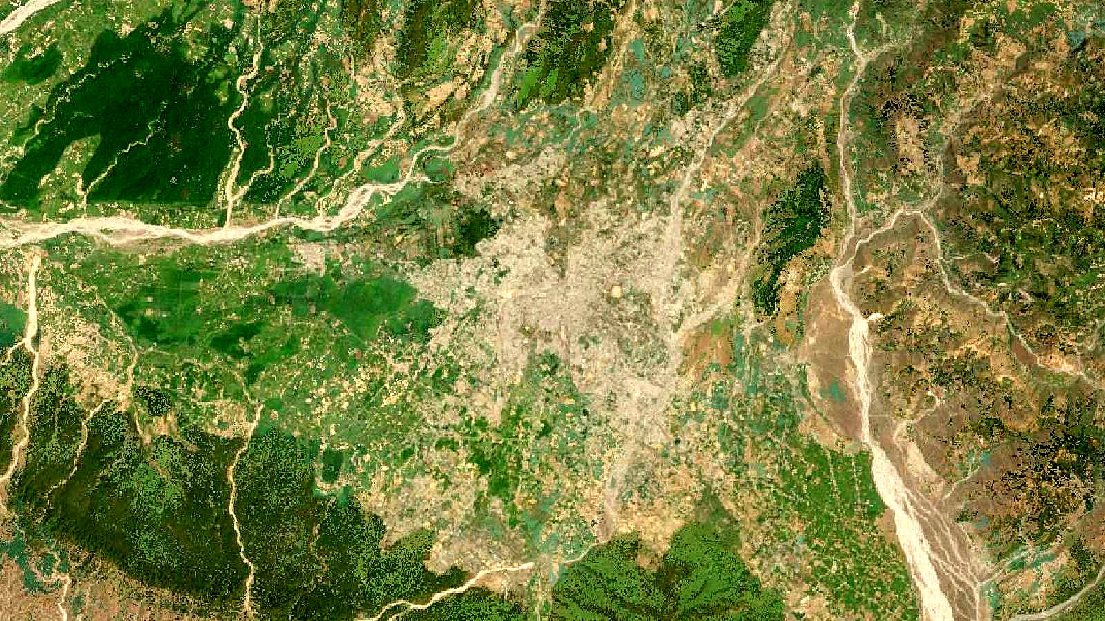
Cover image: Landsat true-colour composite of the Doon Valley, Dehradun (2000), NASA/USGS Landsat WELD via NASA GIBS (public domain).