Why Skipping Radiometric Calibration Costs You Several Degrees

Landsat 8 and 9 carry a Thermal Infrared Sensor (TIRS) with Band 10 centred near 10.9 µm — a spectral window that lets us estimate land surface temperature (LST) from space. The data are freely available through USGS Earth Explorer, and the appeal is obvious: consistent global coverage since 2013, 100 m native thermal resolution resampled to 30 m, and a long archive that predates many competing sensors.

Yet in practice, I regularly see analysts — including students and early-career researchers in India — jump straight from a raw Landsat scene to an LST map without working through the radiometric chain. The consequences are not trivial. Skipping or misapplying calibration steps can introduce errors of several degrees Celsius in your final temperature product. For applications like urban heat island mapping over Delhi or Chennai, agricultural drought monitoring in the Indo-Gangetic Plain, or heat stress assessment during a May heatwave, that kind of error is not acceptable.

This article walks through the full retrieval workflow for Landsat LST retrieval Band 10, explains where errors enter, and gives you a concrete numerical example you can follow in any GIS environment.

---

What Is Actually Stored in a Landsat Band 10 File?

Illustrative: Landsat thermal band urban heat. "Etna Awakens! 🌋" by NASA Goddard Photo and Video is licensed under CC BY 2.0. To view a copy of this license, visit https://creativecommons.org/licenses/by/2.0/.

When you download a Landsat Collection 2 Level-1 product, Band 10 contains Digital Numbers (DNs) — integer values encoding the raw detector output. These are not temperatures. They are not even radiance values yet. The first job is converting DN to Top-of-Atmosphere (TOA) spectral radiance.

USGS provides scene-specific rescaling coefficients in the *_MTL.txt metadata file that ships with every Landsat scene. The conversion is:

L_λ = M_L × DN + A_L

where M_L is the radiance multiplicative scaling factor and A_L is the additive scaling factor, both found in the MTL file under RADIANCE_MULT_BAND_10 and RADIANCE_ADD_BAND_10. The output unit is W/(m² sr µm).

This step is non-negotiable. Using raw DN values as a proxy for temperature produces spatially patterned errors because the scaling factors vary between scenes and even between sensors (Landsat 8 and 9 have slightly different TIRS calibration histories).

---

Converting Radiance to Brightness Temperature

Once you have TOA radiance, you apply the inverse of the Planck function to get Brightness Temperature (BT) — also called TOA BT or satellite temperature. The formula is:

BT = K2 / ln((K1 / L_λ) + 1)

The thermal constants K1 and K2 are also in the MTL file (K1_CONSTANT_BAND_10, K2_CONSTANT_BAND_10). The result is in Kelvin; subtract 273.15 for Celsius.

Important: BT is the temperature the sensor "sees" at the top of the atmosphere. It is not LST. It conflates the actual surface temperature with atmospheric effects and, critically, with the emissivity of the surface. You need two more corrections before you have a usable LST product.

---

The Emissivity Problem — and Why It Matters in India

Illustrative: NDVI vegetation bare soil mosaic. "Public Laboratory NDVI vegetation monitoring" by jeferonix is licensed under CC BY-SA 2.0. To view a copy of this license, visit https://creativecommons.org/licenses/by-sa/2.0/.

Land surface emissivity (LSE) describes how efficiently a surface radiates energy compared to a perfect blackbody. Dry agricultural soils in Rajasthan, dense forest canopy in the Western Ghats, concrete in a Mumbai suburb, and standing water in a Kerala paddy field all have different emissivities in the thermal infrared — typically ranging from around 0.92 for bare dry soil to above 0.98 for dense vegetation and water.

If you assume a uniform emissivity of 1.0 (blackbody assumption), you will systematically underestimate LST over bare and semi-arid surfaces — exactly the surfaces where heat stress and drought research is most critical in India.

The most practical approach for regional studies is the NDVI Threshold Method (NDVI-based emissivity estimation):

1. Compute NDVI from Band 4 (Red) and Band 5 (NIR) of the same Landsat scene.
2. Classify pixels into three categories:
   • Bare soil (NDVI < 0.2): assign a soil emissivity value (commonly ~0.93–0.97 depending on soil type)
   • Full vegetation (NDVI > 0.5): assign vegetation emissivity (~0.99)
   • Mixed pixels (0.2 ≤ NDVI ≤ 0.5): calculate fractional vegetation cover (FVC) and blend soil and vegetation emissivities proportionally
3. Use the derived emissivity layer in the final LST equation

This keeps the workflow entirely within freely available Landsat data — no ancillary emissivity product required.

---

Retrieving LST: The Single-Channel Algorithm

With emissivity in hand, the most widely used approach for single-band thermal data is the Single-Channel Algorithm (sometimes called the radiative transfer equation approach). The simplified form is:

LST = BT / [1 + (λ × BT / ρ) × ln(ε)]

where:

• λ ≈ 10.895 µm (effective wavelength of Band 10)
• ρ = h × c / σ ≈ 1.438 × 10⁻² m·K (a constant combining Planck's constant, speed of light, and Boltzmann's constant)
• ε = surface emissivity from the previous step
• BT = brightness temperature in Kelvin

This formula is an approximation. For rigorous atmospheric correction — especially during monsoon months when atmospheric water vapour over India is high — you should apply a full atmospheric correction using tools like MODTRAN or the Atmospheric Correction Parameter Calculator provided by NASA/USGS, which takes scene acquisition time, location, and atmospheric profile as inputs.

---

A Worked Example: Urban Heat Island in Ahmedabad

Let's say you have a Landsat 9 scene over Ahmedabad acquired in May (pre-monsoon, low humidity). From the MTL file:

• RADIANCE_MULT_BAND_10 = 0.0003342
• RADIANCE_ADD_BAND_10 = 0.1
• K1_CONSTANT_BAND_10 = 774.89 W/(m² sr µm)
• K2_CONSTANT_BAND_10 = 1321.08 K

For a pixel with DN = 22000 (a dense urban surface):

1. Radiance: L = 0.0003342 × 22000 + 0.1 = 7.452 + 0.1 = 7.552 W/(m² sr µm)
2. BT: BT = 1321.08 / ln(774.89 / 7.552 + 1) = 1321.08 / ln(103.6) = 1321.08 / 4.640 ≈ 284.7 K = 11.6 °C

(This is a winter-like value — adjust your actual DN for a May scene where urban pixels routinely reach 315–325 K.)

3. Emissivity: NDVI for this urban pixel = 0.15 → bare/impervious category → ε ≈ 0.95
4. LST: LST = 284.7 / [1 + (10.895 × 10⁻⁶ × 284.7 / 0.014388) × ln(0.95)] = 284.7 / [1 + (0.2155) × (−0.0513)] = 284.7 / [1 − 0.01106] = 284.7 / 0.9889 ≈ 287.9 K = 14.8 °C

The emissivity correction added about 3.2 °C here. Over a high-emissivity water body the correction would be less than 0.5 °C. This is why assuming ε = 1 is dangerous for heterogeneous Indian landscapes.

---

Common Mistakes and How to Avoid Them

• Using Level-1 DN without rescaling. Always apply the MTL coefficients first.
• Ignoring Band 11. Landsat 8/9 has a second thermal band (Band 11, ~12 µm). While USGS advises caution with Band 11 due to stray light issues in the TIRS instrument, some split-window algorithms use both bands. Know your algorithm's requirements.
• Applying a fixed emissivity. Use NDVI-based or land-cover-based emissivity for any landscape with significant bare soil or mixed cover.
• Skipping atmospheric correction in humid months. June–September over most of India has high column water vapour; atmospheric downwelling radiance is not negligible. Use the atmospheric correction parameter calculator for those scenes.
• Mixing Collection 1 and Collection 2 data. USGS updated calibration coefficients between collections. Do not mix them in a time-series.

---

What to Do After You Have LST

A calibrated LST layer opens several downstream analyses:

• Urban Heat Island (UHI) intensity: difference between urban and rural LST in the same scene
• Vegetation health proxies: combine LST with NDVI to compute Temperature-Vegetation Dryness Index (TVDI) for drought monitoring
• Heat stress mapping: overlay LST with population density layers for public health risk assessment during Indian summer heatwaves
• Evapotranspiration estimation: LST is a key input to SEBAL and METRIC ET models used in irrigation management

The key point is that all of these downstream products inherit any error from your LST retrieval. Getting the radiometric chain right is not optional — it is the foundation.

---

References

• USGS Landsat Collection 2 Level-1 Data: https://www.usgs.gov/landsat-missions/landsat-collection-2-level-1-data
• USGS Landsat 8–9 TIRS Band Calibration and Known Issues: https://www.usgs.gov/landsat-missions/landsat-8-tirs-band-quality-assessment
• NASA/USGS Atmospheric Correction Parameter Calculator: https://atmcorr.gsfc.nasa.gov/
• USGS Earth Explorer (data access): https://earthexplorer.usgs.gov/
• Landsat Science: TIRS Instrument Overview: https://landsat.gsfc.nasa.gov/satellites/landsat-9/landsat-9-instruments/tirs-2/

---

Researched with AI assistance and reviewed by Jannat Khosla.

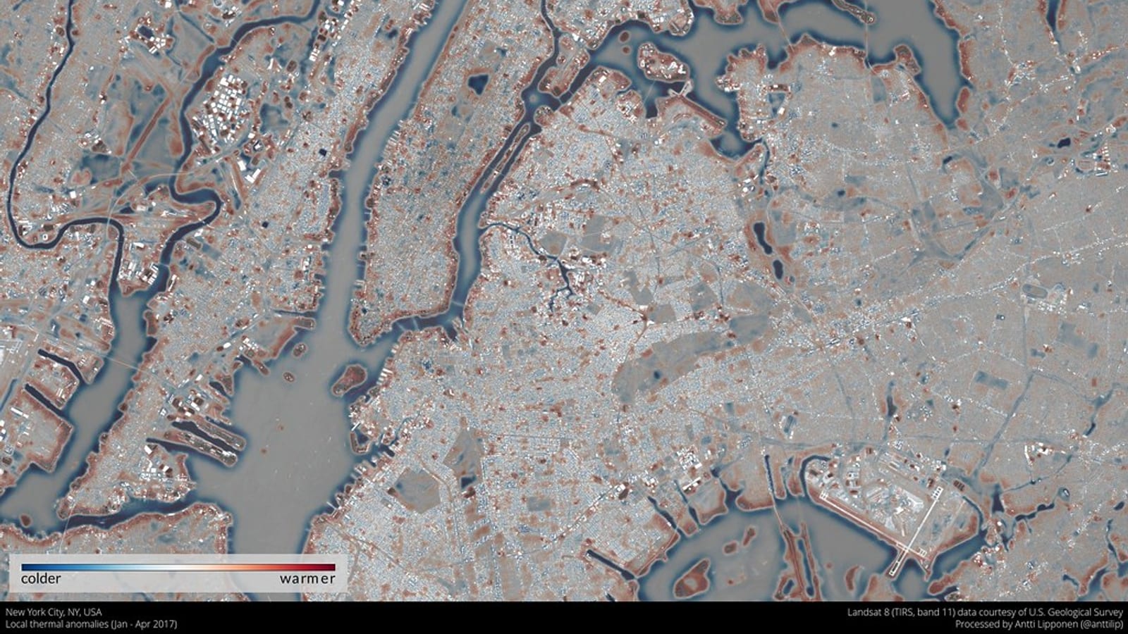
Hero image: "NYC local thermal anomalies Jan-Apr 2017" by anttilipponen is licensed under CC BY 2.0. To view a copy of this license, visit https://creativecommons.org/licenses/by/2.0/.