Network Analysis in QGIS: Shortest Path and Service Area Tools
A practical guide to network analysis in QGIS covering shortest path routing and service area tools, with India-specific data preparation steps, a Nagpur worked example, and guidance on the QNEAT3 plugin for isochrone generation.
Why Indian GIS Practitioners Need This Now
Urban infrastructure in India is expanding at a pace that demands rigorous spatial planning tools. Whether it's a municipal corporation mapping ambulance response zones, a transport planner optimising bus routes in a tier-2 city, or a student completing a capstone project on hospital accessibility, the underlying technical need is the same: reliable network analysis. Commercial GIS software licences remain expensive and often out of reach for government departments working on tight budgets or for students at state universities. QGIS fills that gap, but its network analysis capabilities, particularly the QNEAT3 plugin and the native "Shortest Path" tools, are genuinely underused because practical, India-specific documentation is scarce. This article walks through what these tools do, how to set them up, and how to interpret results meaningfully.
What Is Network Analysis in QGIS, and Why Does It Matter?
Network analysis in QGIS refers to a set of computational methods that treat roads, paths, or any linear infrastructure as a connected graph, nodes (intersections, stops) linked by edges (road segments) with associated costs (distance, travel time, road class). From this graph, you can answer questions like:
- What is the shortest or fastest route between two points?
- Which areas fall within a 10-minute drive of a health facility?
- Where are the critical bottlenecks in a road network?
These are not abstract academic questions. In the Indian context, they map directly onto real planning problems: delineating Primary Health Centre catchment areas under the National Health Mission, planning last-mile connectivity for metro feeder buses, or identifying underserved wards in a Smart Cities Mission project.
QGIS offers two main pathways for this work: the native Network Analysis tools bundled in the Processing Toolbox (available from QGIS 3.x onwards), and the QNEAT3 plugin (QGIS Network Analysis Toolbox 3), which extends those capabilities significantly with isochrone generation and OD matrix computation.
Setting Up Your Network Data
The most common mistake beginners make is jumping straight into the tools without preparing the road network. A few practical steps before you start:
1. Source your road data. OpenStreetMap (OSM) is the most accessible source for Indian cities. You can download it via the QuickOSM plugin directly in QGIS, filtering by highway tags. For official work, some state governments publish road network shapefiles through their GIS portals, though coverage is uneven.
2. Check topology. Network analysis only works if your lines are topologically connected, meaning road segments actually share endpoints at intersections rather than crossing without snapping. Use QGIS's "Check Validity" tool and the "v.clean" tool (from the GRASS provider in the Processing Toolbox) to fix dangling nodes and duplicate geometries.
3. Project your data. Use a projected CRS appropriate for your region. For most of India, UTM Zone 43N (EPSG:32643) or 44N (EPSG:32644) works well, or the national system WGS 84 / India NSF. Avoid running distance-based analysis in geographic coordinates (degrees).
4. Add a cost field. If you want time-based routing rather than pure distance, add a field to your road layer with estimated travel speed per road class (e.g., 50 km/h for national highways, 20 km/h for residential streets in OSM terminology), then compute a time cost: length_m / (speed_kmh * 1000/60) gives minutes per segment.
Worked Example: Shortest Path Between Two Points
Let's say you're working in Nagpur and want to find the shortest road route between the railway station and a district hospital.
- Open the Processing Toolbox → Network Analysis → Shortest Path (Point to Point).
- Set the Vector layer representing the network to your cleaned road layer.
- For Path type to calculate, choose "Shortest" (distance) or "Fastest" (requires a speed field as the cost column).
- Click the Start point field and use the map canvas to click the railway station location. Repeat for the End point at the hospital.
- Under Advanced Parameters, set the Direction field if your data has one-way street information (OSM uses the
onewaytag). For most Indian city datasets, leaving this as bidirectional is a reasonable simplification unless you're working in a CBD with strict one-way systems. - Run the tool. QGIS outputs a line layer showing the route and an attribute table with the total cost (distance in metres, or time in minutes if you set a cost field).
The output is a simple feature you can style, measure, and export. For a student project, this alone is enough to demonstrate spatial reasoning. For a planner, it becomes the basis for comparing multiple facility locations.
Service Area Analysis with QNEAT3
The Shortest Path tool answers point-to-point questions. Service area analysis, "what can I reach within X minutes?", requires the QNEAT3 plugin.
Install it via Plugins → Manage and Install Plugins → search "QNEAT3". Once installed, it appears in the Processing Toolbox under QNEAT3.
The key tool here is "Iso-Area as Polygons (from Layer)":
- Network Layer: your road network
- Start Points: a point layer of your facilities (hospitals, fire stations, bus depots)
- Size of Iso-Area: the cost threshold, say, 5000 metres or 10 minutes
- Iso-Area Interpolation Raster Resolution: controls the smoothness of the output polygon; finer resolution means longer processing time
QNEAT3 works by computing a cost raster across the network, essentially asking "how far along the network can you get from this point?", and then contouring that raster into polygons. The result is an isochrone: a polygon showing all areas reachable within your cost threshold.
For a practical example, run this for all government hospitals in a district using a 30-minute drive-time threshold. Overlay the result with ward boundaries and population data (available from the Census of India). Wards falling outside all isochrones are your accessibility gaps, the areas most underserved by the current facility distribution. This is exactly the kind of analysis that supports evidence-based planning submissions.
Common Errors and How to Fix Them
"No route found" error: Usually a topology problem. Your start or end point may not be snapping to the network. Use "Snap geometries to layer" to snap your point layer to the road network before running the tool.
Isochrones look jagged or unrealistic: Lower the raster resolution value in QNEAT3 (counterintuitively, a smaller number means finer resolution). Also check that your network has no large gaps from missing road segments.
Processing is very slow: Clip your road network to a reasonable study area before running analysis. Running QNEAT3 on an entire state's OSM road network will exhaust memory on most laptops.
Results don't match real-world travel: OSM data quality varies significantly across Indian cities. Dense urban cores (Mumbai, Delhi, Bengaluru) tend to have good coverage; smaller towns may have incomplete or misclassified road types. Always validate against Google Maps or field knowledge before presenting results.
Taking It Further
Once you're comfortable with basic shortest path and service area tools, the logical next steps are OD (Origin-Destination) matrix computation, also available in QNEAT3, which lets you compute costs between every pair of origins and destinations simultaneously. This is useful for school catchment analysis, supply chain optimisation, or transit demand modelling. Combining network analysis outputs with demographic data from the Census or SECC opens up genuinely policy-relevant spatial analysis that is well within reach using entirely open-source tools.
Network analysis in QGIS is not a replacement for dedicated routing engines like pgRouting or OSRM for large-scale production work, but for project-level analysis, student research, and municipal planning tasks, it is more than adequate, and the barrier to entry is low enough that there is no good reason to avoid it.
Frequently asked questions
What plugin do I need for service area (isochrone) analysis in QGIS?
You need the QNEAT3 plugin (QGIS Network Analysis Toolbox 3), installed via Plugins → Manage and Install Plugins. Its "Iso-Area as Polygons" tool generates isochrones showing all areas reachable within a set time or distance threshold.
What coordinate system should I use for network analysis in Indian cities?
Use a projected CRS suited to the region, such as UTM Zone 43N (EPSG:32643) or 44N (EPSG:32644), or WGS 84 / India NSF. Avoid running distance-based analysis in geographic coordinates (degrees).
Why does QGIS give a "No route found" error?
It's usually a topology problem where the start or end point isn't snapping to the road network. Use QGIS's "Snap geometries to layer" tool to snap the point layer to the network before rerunning.
Can QGIS network analysis replace dedicated routing engines like OSRM for large-scale work?
No. QGIS's tools are adequate for project-level analysis, student research, and municipal planning, but they are not a replacement for dedicated routing engines like pgRouting or OSRM in large-scale production work.
References
- QGIS Documentation - Network Analysis: https://docs.qgis.org/latest/en/docs/user_manual/processing_algs/qgis/networkanalysis.html
- QNEAT3 Plugin Repository and Documentation: https://github.com/root676/QNEAT3
- OpenStreetMap Data for India via QuickOSM: https://plugins.qgis.org/plugins/QuickOSM/
- Census of India GIS Resources: https://censusindia.gov.in
- QGIS Official Plugin Repository: https://plugins.qgis.org
Researched and drafted with AI assistance.
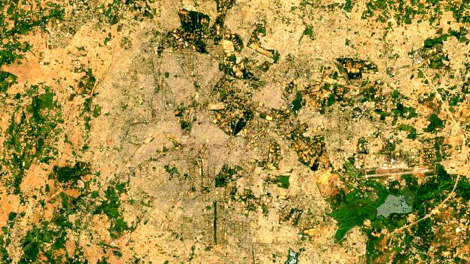
Cover image: Landsat true-colour composite of Bengaluru's road network (2000), NASA/USGS Landsat WELD via NASA GIBS (public domain).