Why Your Classifier Choice Matters More Than You Think

Every time I open a new LULC classification project in Google Earth Engine, the first real decision isn't which satellite — it's which algorithm. Random Forest or SVM? Most tutorials I've seen online just pick one, run it, and declare victory with an 85% overall accuracy. But that number is almost meaningless without context: What was the other classifier's accuracy on the same data? How did each handle class imbalance? How long did each take to train?

This post works through that comparison directly, using LULC classification Google Earth Engine as the framework, with a focus on Indian landscapes where spectral confusion between classes is genuinely hard — think agricultural fallows misclassified as degraded scrubland, or urban expansion eating into peri-urban green cover.

---

What Are We Actually Comparing?

Illustrative: Sentinel-2 false color agricultural mosaic India. "Gabriel y Galán Reservoar, Spain" by SentinelHub is licensed under CC BY 2.0. To view a copy of this license, visit https://creativecommons.org/licenses/by/2.0/.

Before diving into GEE specifics, it helps to be precise about what each algorithm does.

Random Forest (RF) builds an ensemble of decision trees, each trained on a random bootstrap sample of your training data and a random subset of input features. The final class label is determined by majority vote. The key hyperparameters in GEE are numberOfTrees (typically 100–500) and variablesPerSplit.

Support Vector Machine (SVM) finds the optimal hyperplane that maximises the margin between classes in a high-dimensional feature space. In GEE, you access it via ee.Classifier.libsvm(). The critical choices are the kernel type (linear, RBF, polynomial) and the regularisation parameter C. For multi-class LULC problems, GEE's SVM uses a one-vs-one strategy by default.

Both are supervised classifiers. Both need labelled training samples. The differences emerge in how they generalise, how they handle noise, and how they scale.

---

How Do They Behave on Typical Indian LULC Datasets?

Indian landscapes present specific challenges: monsoon cloud cover forces you toward dry-season composites or Sentinel-1 SAR fusion, agricultural calendars create dramatic seasonal spectral shifts, and class imbalance is common (water bodies are often a tiny fraction of the scene).

Random Forest tends to be more forgiving in these conditions. Because it averages across many trees, it handles noisy training samples reasonably well — and in practice, field-collected training data in India often has some positional error due to mixed pixels at field boundaries. RF also gives you variable importance scores out of the box, which is genuinely useful for deciding whether to include a derived index like NDVI, MNDWI, or EVI.

SVM can outperform RF when your training data is small and well-curated. The maximum-margin principle means SVM extracts strong signal even from limited samples, provided you tune the kernel and C correctly. This matters in projects where ground truth collection is expensive — think remote Himalayan districts or restricted forest zones where field visits are difficult.

The practical problem with SVM in GEE is that kernel selection and hyperparameter tuning require iteration, and GEE's server-side execution model makes that iteration slow. You can't easily run a grid search the way you would in scikit-learn.

---

A Worked Example: Setting Up the Comparison in GEE

Illustrative: Google Earth Engine LULC classified map. "TOC Components as shown in Google Earth Engine" by Smithdavid529 is licensed under CC BY-SA 4.0. To view a copy of this license, visit https://creativecommons.org/licenses/by-sa/4.0/.

Here's a minimal reproducible structure for running both classifiers on the same dataset. Assume you have a Sentinel-2 dry-season composite and a training feature collection with a landcover property.

// 1. Prepare composite bands + indices
var composite = s2Median.select(['B2','B3','B4','B8','B11','B12'])
  .addBands(s2Median.normalizedDifference(['B8','B4']).rename('NDVI'))
  .addBands(s2Median.normalizedDifference(['B3','B11']).rename('MNDWI'));

var bands = ['B2','B3','B4','B8','B11','B12','NDVI','MNDWI'];

// 2. Sample training data
var training = composite.select(bands).sampleRegions({
  collection: trainingPoints,
  properties: ['landcover'],
  scale: 10
});

// 3. Train Random Forest
var rfClassifier = ee.Classifier.smileRandomForest(200)
  .train({ features: training, classProperty: 'landcover', inputProperties: bands });

// 4. Train SVM (RBF kernel)
var svmClassifier = ee.Classifier.libsvm({
  kernelType: 'RBF',
  gamma: 0.5,
  cost: 10
})
.train({ features: training, classProperty: 'landcover', inputProperties: bands });

// 5. Classify
var rfMap = composite.select(bands).classify(rfClassifier);
var svmMap = composite.select(bands).classify(svmClassifier);

The key discipline here is keeping everything identical — same composite, same training points, same band stack — so that classifier performance is the only variable. Then run ee.ConfusionMatrix on a held-out validation set for both.

---

Where Each Classifier Tends to Struggle

Random Forest common failure modes:

• Overconfidence in majority classes; minority classes like water or built-up in small towns get absorbed into surrounding agriculture
• Can overfit if numberOfTrees is very high and training samples are few
• Variable importance scores are useful but don't tell you why a feature matters spatially

SVM common failure modes:

• RBF kernel with poorly tuned gamma produces either over-smooth or over-fragmented maps
• Computationally expensive at scale; classifying a large Indian state at 10 m resolution can time out in GEE
• Less interpretable — you can't easily inspect what the model learned

A practical tip I've found useful: run RF first to get variable importance, drop low-importance bands, then feed that reduced feature set into SVM. This often improves SVM accuracy and reduces computation time.

---

Accuracy Assessment: What Numbers to Actually Report

Overall accuracy is the least informative metric for LULC work. For Indian contexts where class imbalance is common, report:

• Producer's accuracy per class (how well you captured each class)
• User's accuracy per class (how reliable the map is for each class)
• Kappa coefficient (though increasingly critiqued, it's still expected in Indian journal submissions)
• F1-score per class, especially for minority classes like water bodies or mangroves

When comparing RF and SVM, look at per-class differences, not just overall accuracy. It's common to see RF win on overall accuracy while SVM does better on a specific class — say, separating built-up from bare soil — because the margin-maximisation in SVM handles that particular confusion better.

---

So Which One Should You Use?

There's no universal answer, but here's a practical decision framework:

• Use Random Forest when: you have moderate to large training samples (500+ points per class), you want interpretability through variable importance, you're working at state or national scale in GEE, or you're iterating quickly on a pilot study.
• Use SVM when: training data is limited and carefully validated, you need strong performance on a specific hard-to-separate class pair, or you're doing a final production run where you can afford the tuning time.
• Consider running both on a subset of your study area first. The accuracy difference is often small, but the pattern of errors is different — and knowing which errors your downstream application can tolerate should drive the final choice.

For most LULC classification Google Earth Engine workflows I've worked on across Indian districts, Random Forest is the pragmatic default. It's faster to tune, scales better in GEE's environment, and produces results that are easier to explain to non-technical stakeholders. But SVM earns its place when the stakes are high and the training data is clean.

The real lesson is: don't pick a classifier because a tutorial did. Run both, compare the confusion matrices class by class, and make the choice explicit in your methodology. That transparency is what separates a credible LULC map from a black-box output.

---

References

• Google Earth Engine Documentation — Classifiers: https://developers.google.com/earth-engine/guides/classifiers
• GEE ee.Classifier.smileRandomForest API reference: https://developers.google.com/earth-engine/apidocs/ee-classifier-smilerandomforest
• GEE ee.Classifier.libsvm API reference: https://developers.google.com/earth-engine/apidocs/ee-classifier-libsvm
• Sentinel-2 MSI User Guide, ESA: https://sentinel.esa.int/web/sentinel/user-guides/sentinel-2-msi

---

Researched with AI assistance and reviewed by Jannat Khosla.

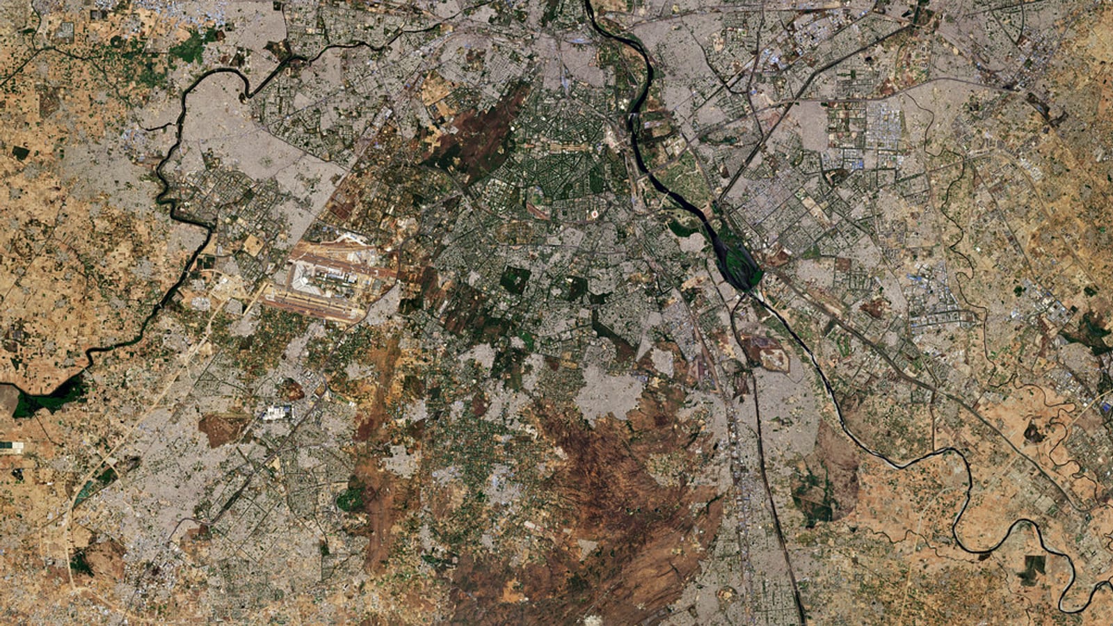
Hero image: "New Delhi, India" by europeanspaceagency is licensed under CC BY-SA 2.0. To view a copy of this license, visit https://creativecommons.org/licenses/by-sa/2.0/.