Watershed Delineation in QGIS Using SRTM DEM: Step by Step
A step-by-step QGIS workflow for watershed delineation using free SRTM 30 m DEM, covering sink filling, flow direction, flow accumulation, stream extraction, and pour-point snapping, with India-specific guidance on where the process commonly fails.
Why Watershed Delineation Still Trips People Up
Watershed delineation is one of those skills that appears in every hydrology and GIS syllabus, yet most tutorials stop at the concept diagram and never walk you through the actual button-clicks. That gap is frustrating, especially when you are a student in India trying to analyse a river basin for a dissertation, or a water-resource professional who needs a quick catchment boundary before a field campaign.
The good news: SRTM DEM covers India at 30 m resolution, it is free, and QGIS with the SAGA provider can do the entire workflow without a licence fee. This article walks through that workflow end-to-end, flags where things commonly go wrong, and explains why each step matters, not just what to click.
What Is Watershed Delineation and Why Does DEM Quality Matter?
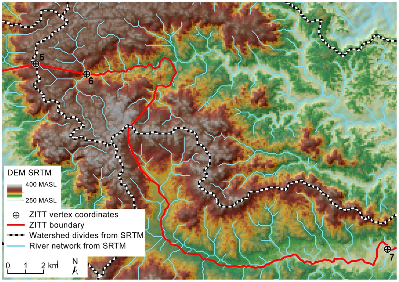
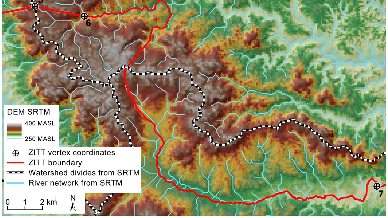
Illustrative: SRTM digital elevation model river basin. "Pone.0066293.g013" by Salvatore Eugenio Pappalardo, Massimo De Marchi, Francesco Ferrarese is licensed under CC BY-SA 4.0. To view a copy of this license, visit https://creativecommons.org/licenses/by-sa/4.0/.
A watershed (or catchment) is the area of land that drains to a common outlet point. Delineating it automatically means asking the software to follow the terrain downhill from every cell until it reaches your chosen pour point.
The quality of that terrain model is therefore everything. As a 2022 study in the Hydrological Research journal shows, a DEM with coarser resolution tends to simulate larger basin areas, shorter streams, flatter slopes, and insignificant differences in altitude, all of which distort your hydrological outputs. A separate accuracy assessment published in Sustainable Futures confirms that DEM accuracy is a critical factor in watershed delineation, water balance assessments, and other geomorphological studies.
A Springer study from 2025 goes further, demonstrating that the choice of DEM significantly influences both watershed delineation and hydrological modelling accuracy. The practical implication: SRTM 30 m is a reasonable starting point for most Indian river basins, but if your study area is a small agricultural watershed (say, a few hundred hectares), you should be aware that stream lengths and slope values may be slightly underestimated compared to what a higher-resolution survey DEM would give you.
Downloading SRTM DEM for Your Study Area
- Go to USGS EarthExplorer or the NASA Earthdata portal.
- Draw a bounding box over your study area in India.
- Under Data Sets, select SRTM 1 Arc-Second Global (approximately 30 m).
- Download the relevant tile(s) as GeoTIFF.
If your basin spans more than one tile, load all tiles into QGIS and use Raster → Miscellaneous → Merge to create a single mosaic before proceeding. Working with a merged, clipped DEM speeds up every subsequent processing step.
The Core Processing Chain in QGIS
The workflow below uses QGIS 3.x with the built-in SAGA provider (available via the Processing Toolbox). All tools mentioned are accessible without any additional plugin.
Step 1 - Fill Sinks
Raw SRTM data contains sinks: cells where water would pool rather than flow out. These are artefacts, not real depressions, and they will break your flow-direction raster if left unfilled.
Processing Toolbox → SAGA → Terrain Analysis – Hydrology → Fill Sinks (Wang & Liu)
Use the filled DEM output for all subsequent steps.
Step 2 - Flow Direction
Processing Toolbox → SAGA → Terrain Analysis – Hydrology → Flow Direction (D8)
The D8 algorithm assigns each cell one of eight cardinal/diagonal directions pointing to the steepest downhill neighbour. This is the standard method for automated watershed delineation and is consistent with the approach used in GIS-and-DEM-based watershed studies such as the IJIRSET 2025 paper.
Step 3 - Flow Accumulation
Processing Toolbox → SAGA → Terrain Analysis – Hydrology → Flow Accumulation (Top-Down)
Each cell now receives a value equal to the number of upstream cells draining into it. High values mark channels; low values mark ridges and interfluves.
Step 4 - Extract Stream Network
Threshold the flow-accumulation raster using Raster Calculator:
"flow_accum@1" >= 1000
The threshold value (here 1000 cells) controls how fine your stream network is. For a 30 m SRTM DEM, 1000 cells corresponds to a contributing area of roughly 0.9 km². Adjust upward for a sparser network or downward for more detail, but be aware that very low thresholds on SRTM data will generate spurious channels in flat areas.
Step 5 - Define the Pour Point
Your pour point is the outlet of the watershed you want to delineate, typically a stream gauge location, a dam site, or a confluence. Create a point shapefile and digitise it precisely on a stream cell in your extracted network. Snapping to the stream raster before placing the point is critical; a pour point even one cell off a channel will produce a nonsensical catchment.
Step 6 - Delineate the Watershed
Processing Toolbox → SAGA → Terrain Analysis – Hydrology → Upslope Area
Input: flow-direction raster + pour-point coordinates. Output: a raster where all cells draining to your outlet are marked. Convert this to a polygon using Raster → Conversion → Polygonize for a usable boundary shapefile.
A Worked Example: Delineating a Sub-Basin of the Godavari
As a brief illustration, consider delineating a tributary sub-basin in Maharashtra. After downloading two SRTM tiles (N19E073 and N19E074), merging them, and running the fill-sinks step, the flow-accumulation raster clearly traces the Pravara River channel. Setting the pour point at the Bhandardara reservoir inlet and running the upslope-area tool produces a catchment polygon of approximately the expected area, a useful sanity check before any modelling work begins.
The JPDS paper on agricultural watershed delineation using SRTM DEM follows a comparable approach for agricultural basins in India, confirming that SRTM-based delineation is operationally viable even where ground survey data are sparse. The GNEST journal study similarly demonstrates that high-resolution satellite-derived DEMs improve drainage network accuracy, which is worth keeping in mind if you later upgrade from SRTM to Cartosat-1 DEM (2.5 m, available through NRSC for Indian study areas).
Common Mistakes and How to Avoid Them
- Skipping the fill-sinks step. This is the single most common reason a flow-direction raster looks patchy or a watershed boundary is obviously wrong.
- Mismatched coordinate reference systems. Reproject everything to a projected CRS (UTM Zone 43N or 44N for most of India) before processing. Working in geographic coordinates (degrees) distorts area and distance calculations.
- Pour point not snapping to the stream network. Always verify visually that your point sits on a high-accumulation cell.
- Using a single SRTM tile when the basin straddles two. Merge first, clip to a buffer around your study area, then process.
- Ignoring coastal or delta areas. SRTM performs poorly in very flat terrain. If your basin is in the Ganga-Brahmaputra delta or a coastal plain, consider supplementing with additional data or manual corrections.
What to Do After Delineation
Once you have a watershed polygon, the typical next steps are:
- Morphometric analysis, compute basin area, perimeter, drainage density, and stream order (Strahler) directly in QGIS.
- Land-use / land-cover overlay, intersect the catchment with LULC data from Bhuvan or Sentinel-2 classifications.
- Runoff modelling, use the catchment as the spatial unit for SCS-CN or rational method calculations.
- Export to HEC-HMS or SWAT, both accept shapefiles and rasters derived from this QGIS workflow.
Frequently asked questions
What resolution is SRTM DEM data, and is it free to use for watershed delineation in India?
SRTM DEM covers India at 30 m resolution and is free; combined with QGIS and its built-in SAGA provider, it supports the entire watershed delineation workflow without any licence fee.
Why do you need to fill sinks before delineating a watershed in QGIS?
Raw SRTM data contains sink cells where water would pool rather than flow out; these are artefacts, not real depressions, and leaving them unfilled breaks the flow-direction raster in later steps.
What flow-accumulation threshold should I use to extract a stream network from 30 m SRTM?
The workflow thresholds flow accumulation at 1000 cells, which on a 30 m SRTM DEM corresponds to roughly a 0.9 km² contributing area. Raise it for a sparser network or lower it for detail, but very low thresholds generate spurious channels in flat terrain.
How does DEM resolution affect watershed delineation accuracy?
Coarser-resolution DEMs tend to simulate larger basin areas, shorter streams, and flatter slopes than reality, which distorts hydrological outputs, so small watersheds mapped with SRTM may show underestimated stream length and slope.
References
- Limits of watershed delineation - DEM resolution effects: https://iwaponline.com/hr/article/53/8/1047/89706/The-limits-of-watershed-delineation-implications
- Open-source DEM accuracy assessment for hydrology: https://www.sciencedirect.com/science/article/pii/S2214581826003277
- Watershed delineation and stream pattern analysis using GIS and DEM (IJIRSET 2025): https://www.ijirset.com/upload/2025/november/21_Watershed%20Delineation%20and%20Stream%20Pattern%20Analysis%20using%20GIS%20and%20DEM.pdf
- Watershed delineation parameters using satellite-derived DEMs (GNEST): https://journal.gnest.org/sites/default/files/Submissions/gnest_04202/gnest_04202_published.pdf
- Statistical evaluation of open-source DEMs for watershed delineation (Springer 2025): https://link.springer.com/article/10.1007/s44288-025-00276-6
- Agricultural watershed delineation using SRTM DEM (JPDS): https://jpds.co.in/wp-content/uploads/2022/07/13.Ramachadran-J-2225.pdf
Researched and drafted with AI assistance.
Hero image: "Pone.0066293.g013" by Salvatore Eugenio Pappalardo, Massimo De Marchi, Francesco Ferrarese is licensed under CC BY-SA 4.0. To view a copy of this license, visit https://creativecommons.org/licenses/by-sa/4.0/.